Econdiscussion
  • Home
  • Articles
  • About Me

Articles

The High Cost of Free Products

16/5/2018

0 Comments

 
​Regulators must look beyond prices to control the anticompetitive behaviour in tech industries
 
“If you’re not paying for it, you are the product,” goes the Silicon Valley saying. While consumers have been enjoying the free products offered by tech firms, Europeans are leading the world in regulating the anticompetitive behaviour of tech companies. The competition commissioner for the European Union, Margrethe Vestager, has established herself as the de-facto worldwide tech regulator.
 
In June 2017, for example, she fined Google €2.42 billion for abusing its market power by redirecting traffic from rival comparison shopping services to its own service, Froogle (which has since been renamed Google Product Search). The press release by the European Commission notes that Froogle entered the market in 2004, but struggled until Google demoted its competitors to the fourth page of search results. Froogle’s competitors consequently received less than one percent of traffic. A key piece of the commission’s argument was that Google’s anticompetitive behaviour harmed consumers. “[Google] denied European consumers a genuine choice of services and the full benefits of innovation,” says Vestager.
 
Other cases of anticompetitive behaviour by tech firms are harder to prove, largely because consumer harm is difficult to establish. According to standard economic theory, monopolies will maximise profit by increasing prices, thereby harming consumers. Thus, regulation is only necessary in the presence of high prices. However, some of today’s tech monopolies, such as Google and Facebook, provide free services, and others, such as Amazon, are operating at wafer-thin profits, suggesting predatory pricing.
 
A monopoly engages in predatory pricing when it prices its products below sustainable levels to drive out competitors, and then raises them back. For instance, Lina Khan, author of the widely acclaimed paper, “Amazon’s Antitrust Paradox,” outlines the story of Quidsi, an e-commerce platform specialising in baby products. After cutting its own baby-product prices by up to 30%, Amazon drove Quidsi to losses, acquired it and eventually scaled back the discounts.
 
Unlike those of traditional industries, the business models of tech companies are often predicated on predatory pricing. Tech companies aim to acquire scale rapidly by forsaking profitability, and investors are willing to finance them only if they can build scale. These unique features of tech companies make it difficult to rely on pricing as the main signal to detect harm to consumers. After all, when the price is zero, how can consumers be harmed? Yet, prices alone do not reflect the harm to consumers caused by less choice and innovation.
 
Another common tactic employed by tech companies is vertical integration, which is the acquisition of one firm in a certain stage of production by another firm in a different stage of production. By itself, it does not necessitate higher prices for consumers, but it does stifle competition. For example, Khan speculates that Amazon might purchase UPS and FedEx such that independent producers of competitive products have no choice but to deliver its products using Amazon. Resultantly, the e-commerce giant can establish itself as a monopoly, not raising prices, but gathering data about its competitors to price its own products more appealingly. Once again, consumers will be harmed by less innovation in the market.
 
The regulatory focus on proving harm to consumers through prices was established in the 1970s and has since become ineffective in promoting competition in tech markets. The repercussions of sclerotic competition are far-reaching as start-ups will be discouraged from entering the market, especially in America, where the focus is still on privacy and not on consumer harm. Regulators must scrutinize the actual harm caused by free products offered by these tech titans – after all, there is no such thing as a free lunch.
0 Comments

PROOF OF THE STOLPER-SAMUELSON THEOREM

20/2/2018

0 Comments

 
As a break from my three-part series on asset bubbles, I will show the proof to the Stolper-Samuelson theorem as shown in this paper.

To read about the Stolper-Samuelson theorem,
click here.

Proof of the Stolper-Samuelson theorem

The Stolper-Samuelson theorem says that in free trade, given two goods, an increase in the price of one good will result in an increase in the return to that good, and a fall in the return to the other good.

There are two proofs to the Stolper-Samuelson theorem provided in this paper. I will be working through the first one.

Part 1: Introduction

Assume two homogenous goods, A and B, and two factors of production, labor and capital (denoted by L and K respectively). Both goods use a mix of labor and capital, but good A is capital-intensive, while good B is labor-intensive.

Part 2: The dynamics between capital and labor in two industries

1. Assume that the amount of labor and capital in the economy are fixed. This will be denoted by L bar and K bar.

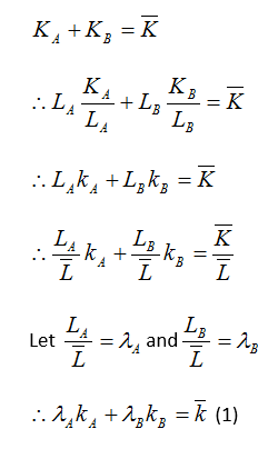
The total labor used in the economy is the sum of the labor used in industry A and the labor used in industry B. The total capital used in the economy is the sum of the capital used in A and B as well, i.e.:
Picture
Picture
2. Now:
Picture
3. Now:
Picture
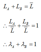
4. The dynamics between labor and capital:
Picture
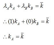
Combining this with (1):
Picture
I.e. when all the labor moves towards sector A, all the capital will move towards sector A as well.

Part 3: Prices, marginal product, wages, and rent

1. Let all the production in the economy be M. Let the price of good A be PA and the price of good B be PB.

Thus:
Picture
Now, we find the marginal products of labor and capital for both goods by finding the partial derivatives.
Picture
Let the price of labor, which is wages, be denoted by w. Let the price of land, which is denoted by rent, be r. Now, if we assume total factor mobility, then wages and rent must be equal (if they are not equal, then all the labor or capital will go to one industry, and there will be no labor or capital in the other).
Picture
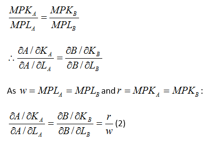
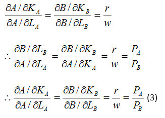
2. Thus, each industry can swap out capital for labor equally as well as the other industry, i.e. the ratio of the marginal products in both industries must be equal:
Picture
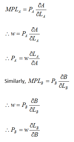
8. Solve for PA and PB:
Picture
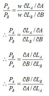
Thus, the price ratio is:
Picture
9. Reworking statement 2:
Picture
Part 4: The Stolper-Samuelson Theorem

When free trade takes place, “trade would reduce the relative price of the import-competing good”, according to the paper. In other words, PB would decrease. As PB decreases, labor and capital moves towards good A, as it is more profitable.

When the price ratio increases, the marginal product of capital in industry A will increase more than the marginal product of capital in industry B, as industry A is capital-intensive, i.e.
Picture
Similarly, when the price ratio increases, the marginal product of labor in industry B will decrease more than the marginal product of labor in industry A, as industry B is labor-intensive, i.e.
Picture
The lower relative marginal products of labor in both industries mean a lower real wage and a higher rent. This is the Stolper-Samuelson theorem.
0 Comments

a world in crisis: are we in an asset bubble?

16/1/2018

0 Comments

 
This series is a three-part exploration on our next financial crisis. The first part explored the fundamentals of a financial crisis, and this second part argues that we are currently in an asset bubble.

According to The Economist, investors do not seem to be worried about an asset bubble, much less a crash. Standard & Poor, a credit rating agency, stated that in advanced economies, the negative bias (i.e. number of bond issuers with negative outlooks) is “at a multi-year low”.
 
Ask Jeremy Grantham, one of the investors who predicted the dotcom boom, and he disagrees entirely. Grantham states, in his publication “Bracing Yourself for a Possible Near-Term Melt-Up (A Very Personal View)” that “a melt-up or end-phase of a bubble within the next 6 months to 2 years is likely, i.e., over 50%”.
 
However, the economy currently shows none of the usual symptoms of a bubble. According to The Economist, Grantham’s own firm sees an annual loss of 2% from American large-cap equities (in fact, the firm sees that, out of all asset categories, only cash and emerging market equities will produce a positive real return). Furthermore, the Purchasing Managers’ Index (PMI) which measures the economic health of the manufacturing sector, indicates that the global economy is improving. As well, according to The Economist, we have yet to see “signs of the kind of late-stage acceleration in share prices that marked American shares in 1929, and 1999/2000 or Japan in 1989.” The biggest sign of a bubble that people watch for, euphoria, is also missing.

In the previous article, I outlined Shiller’s hypothesis that bubbles are exacerbated by euphoria, driven by the media. Consider the cyclically adjusted price-earnings ratio (CAPE), which measures how expensive stocks have become. CAPE suggests that the economy is in a bubble, as it has only been this high twice before: once, during the dotcom bubble; and once during the 1929 bubble.  Accompanied by this bubble, we would expect to see euphoria. Today, however, there is no euphoria, and the media is not exacerbating booms and busts. Why don’t we see euphoria?

According to Grantham, perhaps looking at the usual signs of a bubble will not do us much good. He argues that “we have to reconcile to the fact that no two bubbles, even the classics, are the same. They share the fact that there are many signs of investor euphoria, sometimes indeed approaching the madness of crowds, but the package of psychological and technical indicators has been different each time.”

So, what is different with this bubble, compared to previous ones? Usually, euphoria is linked to a certain asset, such as tech stocks during the dotcom bubble, or property prices during the GFC. However, we see a bull market for almost everything: from stocks, to bonds, to property. They are all expensive compared to their long-term averages. In this situation, it is hard to pinpoint a rise in one asset; resultantly, euphoria cannot take off the same way it did in previous economic bubbles. Consider three assets that are in a bubble: stocks, equities, and property.

The Economist argues that stock prices do not reflect their intrinsic value. CAPE tells us the price of stocks and the extent of overvaluation. Purchasing stock is essentially purchasing a share of profits in a company. Since 1881, the average CAPE for S&P 500 was 17. Now, it is 30. Therefore,  The Economist argues that  “buying a stream of profits is currently uncommonly expensive”. This increase in asset prices is being accompanied by riskier investments that investors do not fully understand any more than mortgage-backed securities (securities that consisted of sub-prime mortgages).

The Economist also notes that equities around the world are also increasing rapidly in price. The S&P 500 index rose by 13% in 2017, which was almost matched by European and Japanese stock markets. European and emerging-market economies’ stock valuations are not as unreasonably high as American ones, but are unambiguously above their long-run averages.

The Economist states that property is also overpriced. In Australia and Canada, two countries who managed to avoid the worst of the GFC, house prices are much higher than their long-run averages, relative to the cost of renting. In America, house prices have risen back above their 2008 peak in nominal terms. They, too, are higher than their long-run average relative to rents. In Britain, there is a similar situation: property prices are nearly at their peak, in terms of average earnings and rents.

We see an asset bubbles in more areas than just stocks, bonds, and equities, such as in credit spreads, according to The Economist. These spreads are the difference between the interest rate offered by safe bonds such as US Treasuries, and by riskier ones, such as bonds issued by companies. According to The Economist, they measure “how much compensation investors require to bear the extra risk”. This spread has narrowed dramatically: people are more willing to take risk for less reward. The Economist points out that in 2016 January, when oil prices sank below $30 and investors predicted a crash in the Chinese economy, the spread for investment-grade bonds was 2.2 percentage points. Now, it is 1 percentage point, which is only slightly higher than the pre-Global Financial Crisis boom. We see a similar story with high-yield or junk bonds.

To make profits, investors look for bonds that are denominated in dollars, but are issued by countries other than America, often emerging-market economies. The Economist argues that the spread between dollar-denominated US bonds and emerging-market bonds has decreased dramatically to 3.1 percentage points in 2017. The Economist continues by pointing out that these bonds bear extremely high risk: in June, many people purchased a dollar-denominated bond issued by Argentina that matures in 2117, despite the fact that Argentina has defaulted six times in the last century, most recently in 2014.

The price increase is not just confined to public markets. The sudden increase in the price of stocks and bonds pushes investors towards private markets, thus pushing prices up there too. The Economist states that investors are particularly looking to funds with a technology bent. For example, SoftBank,  a Japanese telecoms company with sideline in venture capital, has raised $93bn from asset managers to be put into young technology firms.

​Slice it any way possible, and it is hard to deny that the global economy is in an asset bubble. It is not unreasonable to see another crisis on the horizon in the case of wrong policy reactions to this asset bubble. Central banks must tread the line carefully and concoct a policy that deflates this bubble without pushing the economy into a crisis. In the next article, I will explore the role of central banks in financial crises.
0 Comments

A world in crisis: the fundamentals of a financial crisis

23/12/2017

0 Comments

 
This series is a three-part exploration on our next financial crisis. This first article explores the fundamental questions behind the theory of financial crises: what is a financial crisis; what causes it; and why is there an increasing number of them?

According to The Economist, in a recent report on long-term asset returns, Deutsche Bank defines a financial crisis as having at least one of the following four characteristics: a fifteen percent annual decline in equities; a ten percent fall in the currency or government bonds; a default on the national debt; or a period of double-digit inflation. In recent decades, spotting one of the four characteristics has become increasingly easy.

Among the prevalent theories about what causes a financial crisis is Hyman Minsky’s financial instability hypothesis, which argues that overconfidence during times of financial stability inevitably begets financial instability, and this cycle leads to booms and busts. To read more about Minsky’s theory of booms and busts, click here. Along the same lines of placing behavioral factors as the main drivers of financial crises is Robert Shiller’s theory of social contagion of boom thinking. In his book, “The Subprime Solution”, Shiller argues that booms and busts are analogous to a virus, which has a contagion rate and a removal rate (the removal rate is the point where the individual is no longer contagious). Epidemics follow when the contagion rate is higher than the removal rate.

Take, for example, the Global Financial Crisis. Feverish excitement about the property market prevailed in the US, and poorly-backed-up statements such as “property prices have nowhere to go but up” permeated most conversations about property. The prominence of such statements was confirmation of their truth to people. People then disregarded their own judgments and opinions in favor of this general information. Consequently, their contrarian views were never shared with the rest of society, and did not feature in the collective judgement. Thus, over time, the quality of group information declined. Shiller refers to this a feedback loop, in which optimism begat more optimism.

Shiller’s theory of social contagion is further aggravated by herding, where, according to John Cassidy, “at the peak of a bubble, stories of ordinary people getting rich circulate widely, exerting great psychological pressure on others to join the herd”. In a YouTube interview, Shiller elaborates on his point: “We emerged into the 21st century, believing that nothing could go wrong, and so we bought tons of houses. However, the biggest factor is our general complacency.”

The busts were similarly exacerbated by social thinking. At the height of the 2008 crash, nobody knew which bank had exposure to what bad assets, and the overconfidence and hubris that had built rapidly during the boom suddenly turned into to a lack of confidence, which was equally as contagious as the previous build-up of confidence.

Shiller also discusses in depth the role of the media in exacerbating both the booms and busts. For example, in the Global Financial Crisis, the type of stories that interested the media were the ones about poor people getting rich, instead of complicated collateralized debt obligations (CDOs, i.e. sub-prime mortgages that were packaged together and sold to investors). In an essay, Narrative Economics, Shiller explains the role of media in the Great Depression, this time on its crash: “The first narrative of the Great Depression was that of the stock market drop on October 28, 1929. This narrative was especially powerful, in its suddenness and severity, focusing public attention on a crash as never before in America.”

Concrete examples of Shiller’s theory of social contagion during the Global Financial Crisis are abundant. Take, for example, the Icelandic Financial Crisis, and Ireland’s financial crisis. Iceland is a small island and was very closely networked, both socially and politically. There was no one in either politics or business that did not go to the same school or mix in the same circles. This provided a fertile ground for social contagion of thought patterns, which perpetuated the belief that markets could only go up, leading the Icelandic banks to assume ever greater amounts of debt in pursuit of profits. The close interconnectedness of the Icelandic economy meant that the feedback loop was quicker and more vicious.

Ireland, like Iceland, was a small island that was characterized by homogeneity. The small size of the country ensured that politicians and financiers knew each other well, and were thus rendered subject to herd behavior. The media in Ireland exacerbated the boom it faced: it had close ties to the property market, and consequently, huge incentives to keep up property prices. According to Shiller, the media talked up the boom, and the bust was consequently much rougher.

In all previous crises, we have seen telltale signs of financial stability breeding instability, and social contagion causing booms and busts. These have been constant factors in the human nature, but still we see more crises in the last few decades than ever before. Why is there an increasing number of financial crises?

Deutsche Bank argues that the answer lies in the monetary system. Before the early 1970s, when the Bretton Woods fixed exchange rate system was in place, money creation was limited. A country that increased its supply of money too quickly faced inflation. This led to the price of exports increasing, which led to a decrease in exports, which led to exchange rate depreciation, which led the central bank to no longer expand money supply too quickly. In other words, it was hard for financial bubbles to form, given the central bank’s control over money supply.

However, following the abolition of Bretton Woods in the early seventies, most developed countries switched to a floating exchange-rate regime. This new system allows them to not “subordinate other goals to maintaining a currency peg” (to see a central bank’s goals in relation to a currency peg, read this article on the Mundell-Fleming trilemma). This allows for greater trade imbalances, as the currency can bear the burden of it – at least for a while.

These problems are reflected in government debt, which, since floating rate regimes, has been rising as a ratio to GDP. Governments find no pressing reasons to reduce the debt-to-GDP ratio: according to The Economist, “Japan has had a deficit every year since 1966, and France since 1993. Italy has managed just one year of surplus since 1950.” Consumers and companies, as well, have been taking on more debt as well.

This is especially worrying. In previous crises, such as the Global Financial Crisis, debt has financed the purchase of assets to cause an upwards spiral, i.e. a boom, and this similar downwards spiral can happen during a bust. To understand the role of debt in a bust, it is important to understand leverage. Leverage is the degree to which an investor is using borrowed money as opposed to his own funds (equity).

Consider, first, an asset bubble. Assume an asset price goes up. This enables investors to borrow more against the assets, while maintaining the proportion of debt. In fact, encouraged by the rising asset prices, lenders are willing to raise the proportion of debt. With the additional debt available, investors are able to buy more assets, raising the asset prices further in an upward spiral.

A similar process in reverse happens during the deleveraging stage. In fact, the longer the deleveraging cycle persists, the worse the situation gets. During deleveraging, firms usually sell the easy-to-sell assets that are the most liquid. The longer this goes on, the worse the quality and liquidity of the remaining assets.

A sudden fall in asset prices during a deleveraging cycle does not happen randomly: it is often caused by an external event. CNBC refers to the Deutsche Bank report, and cites a multitude of potential triggers for a fall in asset prices, if we are, in fact, in an asset bubble. Among these triggers is a potential Italian crisis. Deutsche states: "A country nearing an election and with high populist party support, with a generationally underperforming economy, a comparatively huge debt burden, and a fragile banking system which continues to have to deal with legacy toxic debt holdings ticks a number of boxes to us for the ingredients of a potential next financial crisis." Other triggers that Deutsche has cited are Brexit, and a rise in populism.

If we are in a bubble, then we can expect to see a bust in the coming years. If this is the case, central banks must have enough tools to protect the economy from this bust. As a reaction to the crisis, in 2008, central banks cut interest rates and bought assets directly in a mechanism known as quantitative easing. This stopped the previous crisis, but each boom and bust cycle has reflected higher debt levels and asset prices. Now we see that the combined valuation of bonds and equities in the developed world is at its record high.
 
If this really is the case, all evidence points to a debt-related boom-and-bust cycle. If we are in an asset bubble, we should be able to see the social contagion of thinking exacerbated by the media, as well as risky investments replacing safe ones. In the next article, I will look at signs that we are currently in an asset bubble, including the prices of stocks, equities, and property.
0 Comments

a world in crisis: introduction

16/11/2017

0 Comments

 
The caution after the Global Financial Crisis has faded away, and in its place is yet another economic bubble. The next few articles will explore how we came to be here, and what our economic outlook is in the next decade. This series uses five articles from The Economist:

1. The next financial crisis may be triggered by central banks
2. The dog that’s yet to bark: Where did the inflation go?
3. Is the bubble only starting?
4. How to spot the next crisis
5. The bubble without any fizz

​In the first article, I explore the fundamentals of financial crises: what constitutes a financial crisis, what causes it, and why we see an increasing number of them. The next article will explore the telltale signs that suggest an economic bubble. The third one will address the central bank as a key economic actor in this coming financial crisis, including an examination of whether the next crisis will be caused by central banks, the role of inflation in determining central banks’ motives, and what policy steps the central bank should take.
0 Comments

What's wrong with QE?

16/4/2017

0 Comments

 
In October 2016 I was asked to give a talk on “What’s Wrong with QE?” to an anti-fractional-reserve-banking organization called Positive Money. I have split my findings on what’s wrong with QE into two sections: fundamental flaws with the theory behind QE, and practical problems with implementing QE.
 
Flaws with the theory behind QE
 
There are a multitude of flaws with the theory behind QE. Three important ones are that QE provides diminishing marginal utility, it decreases a country’s exchange rate, and it assumes that confidence in the program is unfaltering.
 
1. Why does QE provide diminishing marginal utility?
 
David Rosenberg, Chief Economist and Strategist at Gulskin Sheff, summarized why QE provides diminishing marginal utility in the U.S.. All of the arguments cited below apply to virtually any central bank that utilizes QE as a means of economic recovery.
 
  1. Credit growth remains anemic despite massive rounds of QE. My reasoning behind this is that perhaps, at the initial stages of QE, those investors who were hesitant to borrow were galvanized by the low interest rates into borrowing; with more and more rounds of QE, fewer and fewer people borrowed as they had already done so in the past. At this stage, where the sheer volume of investors is no longer high enough to allow banks to make a profit, the extremely low interest rate dissuades banks from lending entirely; interest rates would have to be higher to compensate for diminishing volume of borrowers to allow banks to make a profit.
  2. The “wealth effect” people feel with an influx of money is only permanent if the influx of money itself is permanent. With the UK, talks about winding down the QE program largely dissuaded investment. Thus, increased mentions about winding QE down was met with diminishing utility with QE - people felt poorer and poorer the more winding down was mentioned.
 
2. What is the relationship between QE and exchange rates?
 
  1. A change in the yield due to the increased supply of money in an economy results in a depreciation of the exchange rate to maintain the yield. This is summarized in the chart below.
Picture
It is important to note that none of these figures is factually accurate. These figures were simply imputed to simplify the explanation of the relationship between the exchange rate and the yield. In fact, by definition, the interest rate during QE is much closer to 0% than it is to 1%. Having the interest rate at 1% means this is expansionary monetary policy. Still, we consider 1% to be the interest rate during QE for ease of explanation.
 
Assume that, before the QE program is implemented, a U.S. investor wants to invest $1 in U.K. government bonds. This process takes a few steps.
  1. In Year 0, he exchanges $1 for £1.
  2. He invests £1 in government bonds
  3. In Year 1, he has £1.02
  4. Assuming the exchange rate hasn’t fluctuated, he exchanges £1.02 for $1.02. Thus, his yield is 2% - he has earned 2% over the course of the year.
 
Now, assume that after the QE program is implemented, a U.S. investor wants to invest $1 in U.K. government bonds. For this to happen, he must expect the same yield; otherwise, he will not bother investing. During QE in the U.K., the interest rate has decreased to 1%. To maintain a 2% yield, the interest rate must increase by about 1%. This is why:
 
Assume the interest rate has changed by x%. The investor ultimately wants to make £1.02 from a £1 investment, i.e. a 2% yield. However, the interest rate in the U.K. is only 1%, i.e. the investor will only get $1.01 in Year 1 if he puts in $1 in Year 0. The extra $0.01 must then be made because of an exchange rate change.
 
In other words, $1.01 must now be worth £1.02 to maintain the same yield, i.e. $1.01=£1.02, or $1=£1.01.
 
Why is this a problem? After all, wouldn’t this increase exports and decrease imports, thus improving trade balance? Yes; however, other economies are likely to start a currency war to make their own exports competitive again.
 
In fact, the other problem with different exchange rates globally is that it allows for something called carry trade, a phenomenon in which an investor will borrow money from a country with a low exchange rate and invest in a country with a high exchange rate, pocketing the difference for himself.
 
3. Why is it wrong to assume that confidence in the program is unfaltering?
 
Confidence in the markets differ as different stages of QE are implemented. This one is rather self-explanatory. Depending on how international investors interpret statements made by central banks, it may lead to capital flight or rapid capital influx.
 
Practical problems with implementing QE
 
  1. QE encourages risky investment. Investing in government bonds itself don’t provide a high enough yield. Investors are forced to turn to riskier investments if they want to enjoy higher returns. Ultimately, it starts to sound like a situation that’s very similar to a pre-financial crisis situation: bad investments and risky behavior begets a financial crash.
  2. Banks find it hard to make any type of profit given the extremely low interest rates, and are somewhat dissuaded from lending. This defeats the purpose of QE entirely, where the aim is to encourage banks to lend by influxing the banks with printed cash.
  3. At some stage, central banks might have to start buying other assets such as corporate bonds and even equity shares. This leads to a severe distortion in financial prices and distorts the playing field.
  4. Asset prices increase as a result of QE for two main reasons: First, the increase in money supply for individuals must be put into something. Assets are usually a good bet due to their relative stability. Second, the low prices of assets means that people are encouraged to hold them for longer - after all, why not buy a house if the interest rate is practically 0%?
 
If not QE, then what?
 
Before discussing alternate monetary policy measures, it’s important to revisit the question, “what’s wrong with QE?”. One interpretation might be that this question is genuinely asking about the failures behind QE, some of which have been noted down already. The other interpretation of the question is a more challenging one - “what, exactly, is it that’s wrong with QE?”. Both questions are equally as important. While it is important to recognize the drawbacks of QE, it is equally as important to keep in mind that QE was the saving grace in many economies, especially the U.S.. Just because it poses problems like diminishing marginal utility now, does not mean that the same problems existed at the beginning of the program. Most economists are in consensus that QE is necessary for struggling developed economies. Without it, their economies would be suffering far past what we could imagine.

What alternatives do we have to QE? There are many, but the one most worth mentioning is helicopter money, in which there is increased collaboration between a government and a central bank to target money supply very directly. More about helicopter money will be posted soon.
0 Comments

6. "The Mundell-Fleming Trilemma: Two out of three ain't bad" - The Economist

4/2/2017

0 Comments

 
Synopsis: The last in the series of seminal economics ideas discusses the Mundell-Fleming trilemma, its uses, and whether it actually stands the test of time.

Click here to read the original article.
Discussion:

What is international macroeconomics?

The Mundell-Fleming trilemma is rooted in international macroeconomics, which is the study of policymaking decisions that affect how global economies interact with one another. International macroeconomics deals with issues such as balance of payments, trade agreements, and capital controls.

What is the Mundell-Fleming trilemma?
​

The Mundell-Fleming trilemma is described as the essence of international macroeconomics, according to Michael Klein from Tufts University. It states that, given the choice between monetary autonomy (explained under ‘Context’), free capital mobility, and a fixed exchange rate, an economy can only choose two of them. The trilemma is represented below.
Picture
​Two of the three corners of the triangle can be achieved by any economy; the third must be forsaken. Below is a table showing three different economies and which of the choices they surrendered.
Picture
Forsaking free capital mobility

For example, let’s take an economy that decides to maintain both monetary autonomy and a fixed exchange rate.

Assume the U.K. has its interest rate set at 2% a year, and its exchange rate is at parity with the U.S. dollar, i.e. $1 will get you £1. The U.K. decides to fix its exchange rate such that it is always at parity with the U.S. dollar.
​
Given this scenario, U.S. investors convert $10,000 a day to £10,000 and invest it in the U.K. economy. Now, assume that the Bank of England wants to decrease interest rates in order to encourage British investment in the local economy: the interest rate falls to 1%.
U.S. investors now feel less inclined to invest as much money as their return has decreased by 1%. Thus, they want to convert fewer U.S. dollars into the British sterling, i.e. the exchange rate falls. This is illustrated below.
Picture
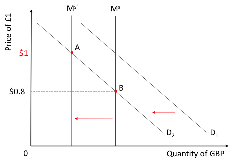
Originally, the Bank of England released an amount Ms of the British pound (GBP) in the international markets. The demand for the GBP, indicated by D1, resulted in an exchange rate of $1=£1. When the Bank of England reduced its interest rate to 1%, the demand for GBP fell from D1 to D2. Resultantly, the exchange rate fell to $0.8=£1. Because Britain has chosen to maintain both monetary autonomy (i.e. it will not increase its interest rate back to 2%) and a fixed exchange rate, it has to forsake free capital mobility by decreasing the money supply to Ms’. In other words, it cannot allow the amount of financial capital, including money flows, to be determined by external forces. Now, the exchange rate is back at $1=£1.

Forsaking a fixed exchange rate

If an economy decides it wants monetary autonomy and free capital mobility, it will have to give up control over its exchange rate. Assume that a certain event in the U.K., such as Brexit, has caused panic amongst international investors. They withdraw their financial capital (such as money) due to uncertainty over the future of the British economy, which depletes the U.K.’s reserves of foreign currency. Without the Bank of England’s increasing interest rates to encourage capital influx, foreign reserves stay low. Without these reserves, the U.K. cannot maintain a fixed exchange rate (explained under ‘Context’), and must allow its exchange rate to float.

Forsaking monetary autonomy

If an economy decides to maintain both a fixed exchange rate and free capital mobility, it must forsake monetary autonomy. To maintain a fixed exchange rate, the U.K. must have a certain level of foreign reserves, i.e. it has to ensure that foreign investors are incentivized to invest in the British economy, which would maintain the level of foreign reserves. If it wants to allow capital to move freely between borders, it must set an interest rate high enough to encourage a certain level of foreign investment. In other words, the U.K.’s interest rate must be determined by the amount of foreign reserves it requires to maintain a currency peg.

An example of a currency peg is the Hong Kong dollar, which, since 1983 has been pegged to the U.S. dollar at a rate of US$1 = HK$7.80. Between 1974 and 1983, the Hong Kong dollar was allowed to float. In 1974, the U.S. dollar depreciated, which encouraged capital influx to the U.S., and consequently, capital outflows from Hong Kong. As Hong Kong chose not to stem capital outflows, it had to choose between allowing its currency to float and forsaking monetary autonomy. Until 1983, it chose the former. To read more about the history of the Hong Kong dollar, click here.

The trilemma and the EU

The Euro was first launched in 1992, under the Maastricht Treaty. In order for an economy to participate in the Euro, it had to fulfill six conditions, one of which was to have an interest rate set close to the EU average. In the run-up to the establishment of the Euro, economies fixed their currencies to the Deutschmark (the currency used earlier in Germany) and allowed their capital to move freely across borders. The participating European economies then relinquished monetary autonomy and followed Germany’s interest rate closely. Wim Duisenberg, the head of the Dutch central bank, was dubbed “Mr. Fifteen Minutes” due to the alacrity with which he copied the interest rate decisions of the Bundesbank, the German central bank.

Today we can see the implications of a single interest rate in the EU. For economies that followed Germany’s business cycle back when the Euro was first established, such as the Netherlands, there was little impact of copying Germany’s interest rate. However, for economies that did not parrot Germany’s business cycle, such as Greece and Spain, interest rates were too low during booms, which caused major troubles when their economies faced busts.

After the Global Financial Crisis (GFC), the EU was hesitant to embark upon QE, a policy that necessitated lower interest rates across the common market. Even though it would have helped the suffering PIIGS (Portugal, Italy, Ireland, Greece, and Spain) economies by encouraging domestic investment, Germany voiced its hesitance, stating that it would leave Germany vulnerable to hyperinflation. Determining an interest rate that placates all members of a common market has proven to be nearly impossible.

The history of the trilemma

The first mention of some tension when it comes to international macroeconomic policymaking was by J.M. Keynes, who, in his 1930 essay “A Treatise on Money”, stated that “[preserving]… the stability of local currencies… and [preserving] an adequate local autonomy for each member over its domestic rate of interest and its volume [poses a dilemma]”.

This dilemma (Keynes assumed free capital mobility­) was the basis of Keynes’ criticism of the interwar gold standard: trade imbalances forced deficit countries to raise interest rates and lower wages to stop the hemorrhage of capital, which led to mass unemployment. If surplus economies increased their imports, this problem would be self-solving, but no surplus economy had any mandate to do so.

In the Bretton Woods conference, Keynes proposed a solution in which an international clearing bank (ICB) aids with deficits and dissuades surpluses. Unsurprisingly, this idea faced great opposition from America, which was an economy with a large trade surplus. The ICB was abandoned, but the idea of an international bank aiding deficit countries became the basis for the IMF.

Marcus Fleming was in touch with Keynes when he wrote his paper on the impotence of monetary policy in the face of a fixed exchange rate and freely-moving capital. Independently, Canadian economist Robert Mundell reached a similar conclusion, but was inspired by different circumstances.

Years after the Second World War, there were scarcely any countries that faced rapid and free capital mobility. Canada was an exception: it allowed capital to travel freely through its border with America. Because it valued monetary autonomy highly, it had no choice but to let its currency float from 1950 to 1962.

Maurice Obstfeld, the current Chief Economist of the IMF, was the first one to mention the term “policy trilemma” in a paper he published in 1997. Since then, the trilemma has become a centerpiece of macroeconomic textbooks, and a conversation piece for international policymakers.

Why the trilemma matters

International trade and globalized economic activity became increasingly commonplace after the Second World War. Economies that had to deal with sudden capital flight or influx, or struggled to maintain control over their currency, had to turn to a previously-ignored idea to not only understand why they did not have as much control over their markets as they did before the war, but also to understand how to deal with it and what the opportunity costs of choosing certain policies were.

The Mundell-Fleming trilemma paved the way for conversation about policymaking with reference to international economies. Today, we notice the impact of all policy decisions on global economic activity: divergence in terms of QE policies between the U.S. and Japan might lead to carry trade; China’s maintaining both monetary autonomy and a strongly-managed exchange rate means that it must employ capital controls; the Bank of England’s decision to continue with QE resulted in a depreciation of the GBP.

A criticism of the trilemma
A big critique of the Mundell-Fleming trilemma has been provided by Helene Rey, from the London Business School, who stated that an economy that allows both capital flows and a floating exchange rate will not necessarily have control over its monetary policy. To hear her lecture on why, click here.

Context

1. What is monetary autonomy?

Monetary autonomy denotes a central bank’s ability to choose its policies, especially interest rates, without taking into account the impact of its interest rate on international markets.
If a central bank has to take into account the reaction of international markets due to an interest rate decision, it would be because higher interest rates would encourage investors to purchase local government bonds, leading to capital influx. Alternatively, lower interest rates would lead to capital flight.

2. Why does a fixed exchange require lots of foreign reserves?

A central bank that wants to peg its exchange rate must meet decreased demand for its currency by lowering the stock of its currency in the forex market, and increased demand by increasing the stock of its currency in the forex market.

To increase the stock of its currency, a central bank must buy foreign currency using its own currency. Conversely, to decrease the stock, it must buy its own currency using foreign currency, which means  that it should have a stock of foreign currency to do so.

An economy must have enough foreign currency in its reserves to have the full flexibility to both buy and sell its own currency. Hong Kong, for example, has a large stock of foreign reserves to maintain its peg to the U.S. dollar. For this reason, speculators do not attack the Hong Kong dollar.
0 Comments

5. "Game Theory: Prison Breakthrough" - The Economist

5/12/2016

0 Comments

 
Synopsis: The fifth in The Economist’s series on seminal economic works discusses the theories behind the Nash equilibrium, how it changed mainstream economics and its relevance outside economics.

Click here to read the original article.
Discussion:

What is game theory?

Game theory describes a situation in which a finite number of players analyze not only his or her own decisions, but also the decisions of the other players, before acting in a way that optimizes his or her utility.

Take the most famous example of game theory, the Prisoner’s Dilemma. In this scenario, two mobsters are held in separate cells, each one being interrogated by a policeman. They are both given the same deal. If both of them confess to the murder individually, they each get ten years in prison. If one of them confesses, then he gets to go free while the other one is imprisoned for life. If neither of them confesses, they both spend a year in jail.
​
The decision diagram is shown below:
Picture
In this diagram, Mobster 1’s payoffs are indicated in blue while Mobster 2’s payoffs are indicated in red. To make a decision about whether or not to confess, they must both consider the other person’s actions. Note that life sentence is indicated by 100 years in prison.

A game theory scenario must satisfy a few conditions:
  1. There are a finite number of players who face a finite number of decisions;
  2. Players are rational, i.e. they will do what is best for them;
  3. Players cannot collaborate to settle on the best outcome.

Nash Equilibrium

The Nash equilibrium describes which scenario the players will settle at. Let us consider the Prisoner’s Dilemma again.

Take Mobster 1. If Mobster 2 confesses, it is better for Mobster 1 to confess rather than not confess, as the former will get him only 10 years in prison while the latter lands him a lifetime. If Mobster 2 does not confess, it is better for Mobster 1 to confess rather than not confess, as the former will let him avoid jail entirely while the latter means he is in jail for a year. Thus, whatever Mobster 2 decides to do, it is in Mobster 1’s best interest to confess.

If we take Mobster 2 now, the reasoning is exactly the same, and it is in Mobster 2’s best interest to confess.

Thus, both mobsters will confess and they will each spend 10 years in prison.

Despite the fact that if they had both not confessed, they would each have received a much lighter sentence, they both did what was best for themselves individually. Herein lies the importance of the Nash equilibrium: the optimal action of an individual does not optimize utility in a society.

Dominant, dominated, and mixed strategies

For only a single Nash equilibrium to exist, there must be either a dominant or a dominated strategy.

A dominant strategy is one where regardless of what the other player decides to do, a certain action is always better for a player. For example, regardless of what Mobster 2 decided to do, it is always in Mobster 1’s best interest to confess.

A dominated strategy is the exact opposite: regardless of what the other player decides to do, a certain action is always worse for a player. In the Prisoner’s Dilemma scenario, not confessing is always worse for Mobster 1.

It is important to note the distinction between a dominant and a dominated strategy. In a two-player game, if there is a clear dominant strategy, then the opposite decision is the clear dominated strategy. However, once a game expands past two players, a dominated strategy might be clear while a dominant strategy is not.

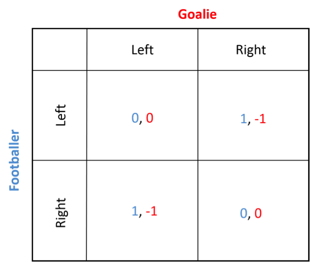
Some games have neither a dominant nor a dominated strategy. These games are called mixed strategy games. Take, for example, a game of football. A footballer who is about to score a goal faces a goalie, who tries to prevent a goal from being scored. This is shown in the decision diagram below.
Picture
Here, there is neither a dominant nor a dominated strategy. Take the footballer trying to score a goal, whose payoffs are indicated in blue. If the goalie dives left, it is in the footballer’s best interest to kick right. If the goalie dives right, the footballer should kick left. There is no dominant strategy.
Similarly, for the goalie, if the footballer kicks left, the goalie should also dive left. If the footballer kicks right, the goalie should dive right. There is no dominant strategy here.

Resultantly, there is no single Nash equilibrium. Instead, we find two Nash equilibria, depending on the decisions each player takes.

Game theory in the real world – Braess’ Paradox

Let us consider a real-world example of game theory: the construction of a highway in a transport system.

Braess’ Paradox holds that, counterintuitively, adding a highway to a transport system will increase travel time for an individual. To read about Braess’ paradox in full, click here. I will be outlining the basics of the paradox.
Picture
Consider a transport system with two highways that take 30 minutes each, regardless of the amount of vehicles on them, and two roads that take x/100 minutes each, where x is the amount of vehicles on the road. To get from A to D, there are two different paths – an individual can either travel through B or C.

Assume 4000 vehicles using the transport system. The Nash equilibrium is that 2000 vehicles would go through route B while 2000 go through route C. Why is this the Nash equilibrium?

Assume 3000 cars go through route B; consequently, there are 1000 cars travelling through route C. It takes people on route B [(3000/100)+30]=60 minutes to get to point D. It takes people on route C [(1000/100)+30]=40 minutes to get to point D. Thus, people on route B will switch over to route C to reduce traveling time.
​
Recall that the Nash equilibrium is when an individual does not want to change their choice of action, as they have nothing to gain from doing so. This will only happen when travel time between the two routes is equal, i.e. when there is an equal amount of traffic on either route. Thus, there will be 2000 vehicles on either route, and it would take them 50 minutes to reach point D.
Now, assume a highway has been added between point C and D, as illustrated below:
Picture
Now, assume that travel time on the highway is 0 minutes (this is, of course, an exaggeration). Let us assume that the highway is being used. Thus, to travel from A to D, an individual has two choices:

A to B, B to C, and then C to D, or A to C, C to B and then B to D.

Let’s consider the former with 1000 vehicles. It would take everyone [(4000/100)+0+(4000/100)]=80 minutes to get to point D.

For the latter case, it takes [30+0+30]=60 minutes to get to point D. Thus, individuals will choose to travel from A to C to B to D.

Now, some vehicles will choose to take the first path, while others take the second. The Nash equilibrium will be when the time travelled in both paths is equal, i.e. it takes 60 minutes to travel by either path.

This will happen when there are 300 vehicles on the first path. Note, however, that the use of the highway has increased travel times for all individuals by 10 minutes.

Why the Nash equilibrium matters

The Nash equilibrium assumes many things, including rational behavior and an ability to successfully predict a player’s payoffs. The biggest thing it assumes, however, is perfect information. In other words, a player knows exactly how another player will act given any scenario in the game. This, of course, is not the case in reality.

The Nash equilibrium has been adjusted by many others since John Nash himself. One revision includes uncertainty about people’s payoffs. Another includes the knowledge of non-credible threats, i.e. knowing whether another player will actually act in a certain way or whether he is just claiming that he will.

Despite all its flaws, the Nash equilibrium is one of the more revolutionary findings in economics for a few reasons. Firstly, the Nash equilibrium shows that individuals do not just weigh their own costs to maximize utility – they look at other players in the market to do so as well. Secondly, it shows that a utility maximizing individual does not necessarily maximize utility for a society. In perfectly competitive markets, for example, an individual’s choice of selling their product for the price at which it costs to produce it maximizes utility not only for the seller, but for the collective market as well.
​
The third way in which the Nash equilibrium is important is through the lens of government policy. Take a game theory scenario in which the dominant strategy for an oil company is to pollute a river. Taxation, or other methods of decreasing the payoff, shifts the company’s dominant strategy to not polluting at all. In this way, the Nash equilibrium is another way to view equilibrium analysis.
0 Comments

4. "Fiscal multipliers: Where does the buck stop?" - The Economist

9/10/2016

0 Comments

 
Synopsis: The fourth in The Economist’s series on seminal economic ideas discusses the relevance and usefulness of the fiscal multiplier.

Click here to read the original article.
Discussion:

Introduction

The idea of the fiscal multiplier was first introduced after World War 1, and has since gained and lost popularity. Now, when economies around the world are debating the usefulness of fiscal stimulus in the face diminishing effectiveness in using monetary stimulus, economists have gone back to the age-old debate: are fiscal multipliers real?

The fiscal multiplier

The mathematics of the fiscal multiplier will be explained under ‘Context’.

The multiplier explains a scenario in which an initial increase (or decrease) in government spending will increase (or decrease) national income by a disproportionate amount.

For example, if the government spends money to build a new school, construction workers, architects, building planners, etc. will be involved in building it. Later, new teachers, janitors and other staff would get hired. The people involved in either building or running the school would then spend some (not all) of the money on other goods and services, such as restaurants. Now, people working at the restaurants have more income, and they can spend some of it on other goods and services, and so on. Thus, the initial action of increased government spending benefits the economy in many ways. The question is to what extent is the accumulated benefits of the successive waves of spending exceed the initial government expenditure.

History of the fiscal multiplier: the 1920s

Many times, the idea is credited to JM Keynes himself, but it was his student, Baron Kahn, who first mentioned it. In the late 1920s the U.K. had slipped into a recession, as World War 1 had caused a depreciation in the pound, while inflation was high. To counteract a low pound, the Bank of England maintained tight monetary control (explained under ‘Context’). This, in turn, created a period of persisting low growth and deflation – the Great Depression.

Many economists had suggested public investment to increase employment in the economy. This idea was unsurprisingly met with resistance from the government, which echoed the U.S. Treasury’s view: public spending would crowd out private spending (to read more about the crowding-out effect, click here), and thus would not help the economy. In fact, it might exacerbate the depression.
​
Baron Kahn argued vehemently against the “Treasury view”, stating that public investment would increase output not only from the primary spending, but also from “beneficial repercussions”.

The Keynesian multiplier and “General Theory”

Unsurprisingly, Kahn’s view was in line with that of his teacher. In his seminal work, “The General Theory of Employment, Interest and Money” (“GT”), Keynes described exactly how the multiplier would boost growth. Because of not only his thorough description of the concept, but also his influence globally, the fiscal multiplier is often referred to as the “Keynesian multiplier”.

GT was, and continues to be, one of the greatest pieces of economic writing. Keynes’ motivation to write the book stemmed from his frustration with the Treaty of Versailles: he lampooned key figures for not considering what he believed were large risks with the agreements set out in the treaty. Keynes, as well, was very unhappy with what was then considered common and accepted economic knowledge, i.e. classical economics (explained under context). Both these factors drove him to write what would be his magnum opus: GT.

It is in GT that Keynes describes the mechanism through which government spending would have secondary effects, which would lead to tertiary effects, and so on. He also states that during a recession, individuals would be more inclined to save than invest; thus, demand for investment would decrease. As a result, an increase in demand for investment from the government should not cause a crowding-out effect.

History of the fiscal multiplier: the 1920s to the 1960s

The success of the theory of fiscal multiplier seemed to be self-evident during the Second World War and for a long time after. The Great Depression prompted economies worldwide, especially the U.S. and the U.K., to adopt Keynesian economics, and the fiscal multiplier. As the governments eventually increased military spending in the course of  World War II, their economies emerged from depression. Reverence of the multiplier increased multifold after, leading Milton Friedman to state, “We’re all Keynesians now”.

History of the fiscal multiplier: the 1970s

It was Friedman himself who began the long line of criticisms of the multiplier. He outlined the relationship between the business cycle and the money supply in an economy, and thus stated that controlling the money supply was all that was needed to control an economy; the multiplier was not necessary at all.

A more fierce line of criticism stemmed from economists belonging to the “rational expectations” school of thought, led by Robert Lucas. They claimed that the multiplier does not exist. Forward-looking individuals would realize that fiscal expansion today would have to be met with fiscal consolidation in the future to stabilize debt: thus, they would save the money they get from the government for when there is an increase in taxes in the future. Thus, there would be no multiplier effect. This idea is dubbed “Ricardian equivalence” (discussed under ‘Context’).

History of the fiscal multiplier: post-1970s

Governments tried fruitlessly to boost economic growth through government spending. Yet, they found that despite quiescent unemployment, inflation and interest rates rose unsustainably. The economic situation post-70s gave rise to a school of economic thought dubbed the “freshwater” school (these economists were named as such due to their proximity to the Great Lakes in the U.S.). They fought to recreate macroeconomics from individual consumers’ actions, a phenomenon named “microfoundations of macroeconomics”.

Robert Lucas’s and Tom Sargent’s work on the criticisms of Keynesian economics won them the Nobel Prize, and the fiscal multiplier quickly lost popularity and pertinence.

Then came the rise of “New Keynesian” economists, most of whom came from near America’s coasts; thus, they were dubbed “saltwater” economists. Notable saltwater economists include Larry Summers, Stanley Fischer and Greg Mankiw. New Keynesian economists believed that “recessions were market failures that could be fixed through government intervention”. However, they placed more importance on the central banks’ management of inflation, unemployment and interest rates than they did on fiscal policy. Thus, the fiscal multiplier once again faded into the background.

History of the fiscal multiplier: the 1990s to now

Developing countries around the world have been seeing little success in central bank policies, especially quantitative easing. Since the 1990s, inflation has remained close to being non-existent in Japan despite the Bank of Japan’s best efforts. Cutting interest rates to zero has not been as successful as any economy had hoped. This led to the resumption of the conversation about fiscal expansion. After the Global Financial Crisis (GFC), the U.S. had secured an $800bn stimulus package to revive its economy.

Freshwater economists argue that during times of panic, economists have resorted to the comforting idea of fiscal expansion, even when it doesn’t work. Other economists argue that the lack of fiscal stimulus after the GFC has damaged economies worldwide. Only time will tell which side of the argument is correct. The only thing that seems clear to economists now is that the argument about Keynes’ multiplier will never end.

Recent experiences or evidence

Fiscal multiplier has been calculated to be greater than one for many developed economies. This means that fiscal expansion will boost the economy past its primary effects, while austerity (fiscal consolidation) will harm the economy more than the initial amount of contraction.

In the EU: Austerity has been a centerpiece of government policy ever since the GFC. In the UK, former Prime Minister David Cameron mentioned the “age of austerity” in a 2009 speech to the Conservative Party. In March, the ex-Chancellor of the Exchequer George Osborne mentioned further government spending cuts of about £4bn. Austerity measures in the EU are well-summarized by this website. Some economists believe that it is excessive austerity measures across Europe that keep struggling economies from a full recession, and that the UK only escaped the recession after austerity measures were loosened.

In Japan: Prime Minister Shinzo Abe has been discussing his “three arrows” to economic recovery for a long time: monetary expansion, fiscal expansion and structural reforms (such as encouraging women to participate in the labor force). However, fiscal expansion has been constantly negated at least partially by increased taxation of sorts, including consumption tax and sales tax.

In the U.S.: The U.S. government, under President Barack Obama, had secured an $800bn fiscal expansion package after the GFC. This, along with QE, did well to aid the economic recovery from the recession. However, many economists such as Larry Summers argue that the fiscal expansion package was not large enough and a larger one would have pulled the U.S. out of recession much quicker.

Context
  1. What is the fiscal multiplier?

Assume a closed economy (i.e. one where there are no imports and exports). The output, denoted by Y, in the economy comes from three sections, each of which can be modeled as follows:
  1. Consumption, denoted by C. Consumption is written as , where:
    • c0 is consumer confidence. The more confident a consumer is in the economy, the more the consumer will consume, i.e. the higher c0 is.
    • (Y – T) is the disposable income. Y is the income a consumer earns, and T is the tax rate. Note that output is the same symbol as income. The intuition behind this is that all the income earned in an economy will finally be spent in the market, i.e. all the income will result in output. Thus, in this model, income = output. (Y – T) is then the disposable income for a consumer, i.e. the income a consumer can spend in the economy after taxes.
    • c1 is the marginal propensity to consume (MPC). This is the share of disposable income that the consumer will actually spend in the economy. Whatever the consumer does not spend, he or she will save. For this reason, MPC is a figure between 0 and 1.​
  2. Investment, denoted by I. Investment is written as , where:
    • b0 is business confidence. The more confident a business is in the economy, the more the business will invest in the economy, i.e. the higher b0 is.
    • b1Y is the proportion of output that leads to investment. In other words, a business that needs to make more and more output will invest more and more in machinery and other things. b1 denotes the proportion of increased output that results in increased investment. b1 always between 0 and 1.
    • b2i is the amount by which an increase in interest rate results in a decrease in investment. If interest rates increase in an economy, it gets more expensive for a firm to borrow money to use in investments, such as machinery.
  3. Government spending, denoted by . The bar above the G denotes that government spending is exogenous, i.e. not determined by the market, but determined by the government itself.
​
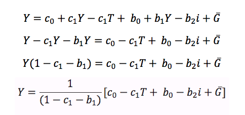
Together, then, total output (or GDP) in an economy is:
Picture
​Rearranging for Y on one side:
Picture
The fiscal multiplier is 1/(1-c1-b1). Thus, whatever happens to any term within the squared brackets, which we call autonomous spending, e.g. if government spending goes up or if taxes go down, Y will be affected through the fiscal multiplier, which would increase the effects of an increase in government spending or a decrease in taxes.

2. Why would the Bank of England’s maintaining tight monetary control counteract a low pound?

Tight monetary control means less money supply, which would keep both interest rates and currency value high.
​
Reducing the money supply in the domestic economy increases interest rates. This is demonstrated in the diagram below.

Picture
In this diagram, demand for money is denoted by D, and the original supply of money is M1. At the intersection of M1 and D, the quantity of money supplied is Q1, and the interest rate is i1. When the central bank reduces the stock of money, from M1 to M2, the quantity of money reduces to Q2, and the interest rate increases to i2, at the new equilibrium.
​
In the international market, reducing the stock of money increases the currency value. This is shown in the diagram below.
Picture
The demand for the British pound is denoted by D, and the original supply of the pound is S1. The equilibrium price and quantity of the pound at this equilibrium is P1 and P2 respectively. When the central bank reduces the amount of money supplied in the international markets, i.e. decreasing S1 to S2, at the new equilibrium, the quantity of pounds traded decreases to Q2 while the price increases to P2. Thus, the exchange rate increases.

3. Why was Keynes unhappy with classical economics?

Classical economists believed that the labor market is self-correcting, in that people who were not employed did not want to be employed. In other words, there is no such thing as involuntary unemployment.
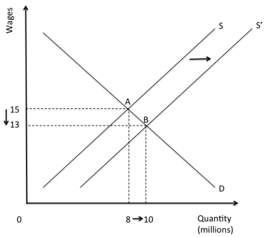
Picture
Consider a simple supply and demand diagram for the labor market, where S is the supply of labor and D is the demand for labor by employers. At the given market equilibrium, A, 8 million people are hired at a price of $15 an hour. Assume more people want to be hired, i.e. the supply of labor increased from S to S’. The new equilibrium is at point B, where 10 million people are hired. However, all laborers now get paid more, at $13 an hour.

This classical model of the labor market suggests that the economy can freely expand and contract to accommodate more or fewer workers, with no problem at all. This was the basic idea that Keynes disagreed with.

Keynes, instead, believed that individuals were more likely to accept more nominal wages rather than less nominal wages, even if their real wages did not change. In other words, prices of labor in the economy do not adjust as easily as classicists believed. He called this the “sticky wage” theorem.

Nominal wages is just the amount of money individuals earn. Real wages are adjusted to inflation. Now, suppose inflation in the economy increased by 2%, i.e. everything cost 2% more. Wages would increase by 2% as well. The individual who receives higher nominal wages is not richer by real terms, but is still happy. However, suppose there is 2% deflation in the economy, i.e. everything costs 2% less. An individual would be much less willing to receive a 2% pay cut, even if he or she remains equally as rich in real terms after the wage cut. Thus, wages are sticky downwards.

4. What are the problems with Richardian equivalence?

​Ricardian equivalence requires that individuals are forward looking: they will save now for a future tax increase. However, few individuals are actually that forward looking, and those who are will not be able to accurately pinpoint when taxes will increase in the future. Thus, if individuals get a boost to their incomes due to higher government expenditure, they are more likely to spend at least a part of the increased income now and worry about tax increases later.
0 Comments

3. “An Inconvenient Iota of Truth” – The Economist

4/9/2016

0 Comments

 
Synopsis: The third in the series discusses the Stolper-Samuelson theorem and how it changed the debate about free trade.

Click here to read the original article.

1. Click here to read the introduction post.
2. Click here to read the first post on asymmetric information.
3. Click here to read the second post on the financial-instability hypothesis.
Discussion:
 
The Stopler-Samuelson theorem discusses the relationship between trade and wages. The theorem suggests that free trade is not always a mutually beneficial scenario.
 
Stolper and Samuelson
 
Wolfgang Stolper was an American economist best known for his work on the Stolper-Samuelson theorem. Paul Samuelson is one of the most celebrated economists and is hailed the father of neo-Keynesian economics.
 
Free trade, comparative advantage and the Heckscher-Ohlin model
 
Free trade is usually seen as a mutually beneficial scenario. This idea can be traced back to classical economist David Ricardo, who is well-known for his work on comparative advantage (explained under ‘Context’). Comparative advantage is seen as a solution to the labor scarcity problem, where some countries do not have enough labor for a certain industry, and some countries have too much. Heckscher and Ohlin together advanced the comparative advantage theory, stating that the country that faces labor scarcity (in the Heckscher-Ohlin model, this country is the U.S.) should specialize in those industries that require little labor, and leave the industries that require lots of labor to other countries that find no shortage of workers.
 
Most economists believe that workers, as well, would be better off from free trade. Some people argued that scarcity gives workers more bargaining power; eliminating scarcity would leave workers worse off as their nominal income would decrease (explained under ‘Context’). However, nominal income would also increase due to free trade, as would purchasing power (explained under ‘Context’). Thus, free trade benefits workers as well.
 
Further, labor has the benefit of being versatile. Thus, if one industry relies more on capital and less on labor, in the long-run, workers can always move to another industry that is more labor-intensive.
 
In both the comparative advantage theory as well as the Heckscher-Ohlin model, both countries and workers participating in trade are better off. Thus, conventional economic wisdom is that free trade is always mutually beneficial.
 
The Stopler-Samuelson theorem
 
Stopler and Samuelson both disagreed that free trade is always beneficial for workers.
 
While he worked in Nigeria, Stopler noticed that textile workers were usually too tired, inexperienced or sick to work productively; consequently, the industry required a 90% tariff to compete (explained under ‘Context’). He lamented about the quality of labor there, stating that if such a high tariff was needed, it wasn’t worth having the industry at all. This was the basis for the Stopler-Samuelson theorem.
 
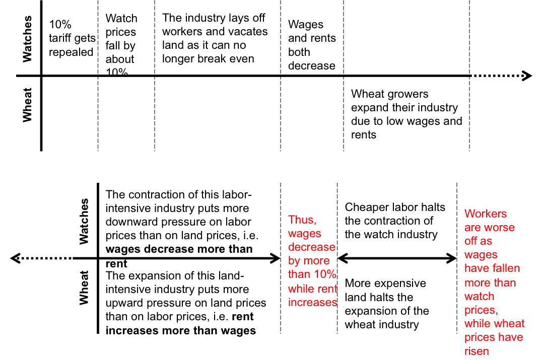
Consider a country that has lots of land but little labor. The country makes only watches and wheat, where the former is labor-intensive and the latter is land-intensive. Suppose the watch industry has a 10% tariff to compete. The Stolper-Samuelson theorem says that if the tariff gets repealed, workers will suffer. The theorem is demonstrated in the timeline below.
Picture
Looking further
 
Variations on the theory include splitting workers into skilled and unskilled labor in an industry, say, watches. The dynamics work similarly: free trade decreases the prices of watches, and the unskilled workers’ wages decrease while the skilled workers’ wages increase.
 
What the Stolper-Samuelson theorem is missing
 
The Stolper-Samuelson theorem does not answer a multitude of questions. For example, the assumptions of the Stolper-Samuelson model are questionable. First, it is a large assumption that a country produces everything, e.g. watches and wheat. Some countries might just produce watches, and some might just produce wheat.
 
The theorem also assumes that both markets are perfectly competitive, and that there are constant returns to scale. Not many industries follow those assumptions.
 
The importance of the Stolper-Samuelson theorem
 
Undoubtedly, the theorem is not directly applicable; given its multitude of assumptions, the theorem in its simplest form is only pertinent in a few circumstances. Stolper himself treated the theorem with great caution, stating that it is only a “slight theoretical possibility” and that many other economists would look at “more realistic concerns”. So why is this theorem so groundbreaking?
 
The theorem shows that free trade is not always beneficial. Economists had earlier approached the topic of free trade with the attitude that nobody would lose. The Stolper-Samuelson theorem shows that free trade does not always have winners. The theorem is an inconvenient iota of truth to those who insist on looking only at the benefits of free trade.
 
Extra reading
 
To read a real-life example of the theorem, click here.
 
While there is no free version of the original paper online, you can access it here for US$40.
 
Context
 
1. What is comparative advantage?
 
To understand comparative advantage, it is important to understand absolute advantage first.
 
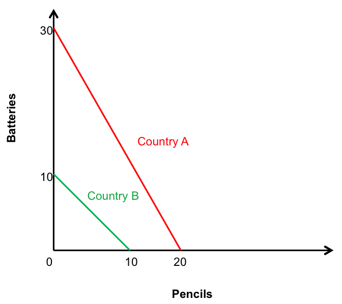
Assume two countries, A and B. Both countries produce batteries and pencils. In one hour, A can produce 30 batteries or 20 pencils. In one hour, B can produce 10 batteries or 10 pencils.
 
Regardless of whether A produces batteries or pencils, it will produce more of them than B can. Thus, A has the absolute advantage over B. This is illustrated in the diagram below.
Picture
​The green and red lines indicate a country’s production possibility curve (PPC). A PPC is any combination of two goods a country might produce. So, A might produce 30 batteries and no pencils, or 20 pencils and no batteries, or some combination of batteries and pencils.
 
As a general rule, a country that has a PPC lying completely above another country’s PPC has an absolute advantage in production.
 
Comparative advantage looks at the opportunity cost of producing batteries or pencils for either country. In this example, A can produce three times more batteries than B can, and two times more pencils than B can. Thus, A should produce only batteries as it is more efficient in producing batteries, i.e. it has the comparative advantage in batteries. As David Ricardo said, the country should produce what it is “most better” in. B should produce only pencils as it is the “least worse” in producing them.
 
A and B would then trade to get whatever quantity of batteries and pencils they require. If they do so, then both countries would get more of each good than if they did not trade.
 
With comparative advantage, A will produce 30 batteries, and B will produce 10 pencils. Totally, 40 goods will be produced.
Without comparative advantage, assume A makes 10 pencils and 15 batteries, and B makes 5 pencils and 5 batteries. Totally, 35 goods will be produced. In fact, if we take any two points on both PPCs, total production will be less than if both countries specialized using comparative advantage.
 
2. Why would scarcity provide workers with more bargaining power, and why would less bargaining power decrease a worker’s nominal income?
 
Scarcity is an extremely important bargaining tool. Suppose, in an industry, there are 100 employers and 5 employees, i.e. employees are scarce. If one employer offers an employee $50 a day, another employer, desperate for that employee, will offer them $70 a day, and so the price of the employee will be bid upwards.
 
Suppose, in another industry, there are 100 employees and 5 employers, i.e. employees are abundant. If one employee offers to work for $50 a day, another employee, desperate for a job, will offer to work for $30 a day, and the price of the employee will be bid down.
 
Thus, scarcity gives you bargaining power, in that workers can ask for more money, and less bargaining power bids a worker’s nominal income down.
 
3. Why would free trade increase a worker’s purchasing power?
 
Purchasing power is how much someone can buy for a fixed amount of money. For example, imagine that in Country A, with US$1, you can buy five chocolates. In Country B, with US$1, you can only buy two. Workers in Country A thus have a higher purchasing power.
 
Assume free trade does reduce a worker’s nominal wages as their bargaining power decreases. But the price of imported goods would also decrease. So the workers would be able to buy more of those imported goods with their wages, i.e., their purchasing power increases.
 
4. What does it mean that an industry requires a 90% tariff to compete?
 
In Nigeria there was a 90% tariff in the textile industry. That means that imported textiles had to pay 90% import duties to the government before they could be sold in Nigeria. Hence the domestic producers could price their products 90% higher and still compete with imports.
0 Comments
<<Previous

    Categories

    All
    Abenomics
    Adam Smith
    Adverse Selection
    Ageing
    Amazon
    Arrows
    Arthur Okun
    Asset
    Asymmetric Information
    Ben Bernanke
    Booms And Busts
    Braess' Paradox
    Brazil
    Bretton Woods
    Brexit
    Bubble
    Bull Market
    Business Cycle
    Capital Control
    Capital Flows
    Capital In The Twenty First Century
    Capital In The Twenty-First Century
    Carry Trade
    Causation
    Central Bank
    China
    Christopher Sims
    Classical Economics
    Consumption
    Counter-cyclical
    CPI
    Creative Destruction
    Crisis
    Daron Acemoglu
    David Cameron
    David Ricardo
    Debt
    Debt-to-GDP
    Deflation
    Deleverage Cycle
    Demography
    Devaluation
    Developing Economies
    Development
    Diffusion
    Diminishing Returns
    Dominant Strategy
    Dominated Strategy
    ECB
    Economic History
    Economic Theory
    Equality
    Equitity
    Equity
    Equity Investments
    EU
    Exchange Rate
    FDI
    Fed
    Federal Reserve
    Finance
    Financial Crisis
    Financial Instability Hypothesis
    Financial-instability Hypothesis
    Financial Times
    Fiscal Multiplier
    Fiscal Policy
    Fixed Exchange Rate
    Fleming
    Floating Exchange Rate
    Free Market
    Free Trade
    Freshwater
    Game Theory
    GDP
    George Akerlof
    Germany
    GFC
    Gini Coefficient
    Global Financial Crisis
    Globalization
    Government Intervention
    Government Spending
    Great Depression
    Growth
    Heckscher-Ohlin
    Helene Rey
    Hyman Minsky
    ICOR
    Illiquid
    Immigration
    Income
    Inequality
    Inflation
    Infrastructure
    Innovation
    Interest Rates
    Investment
    Italy
    James Robinson
    Janet Yellen
    Japan
    Jean Tirole
    J.M. Keynes
    John Nash
    Keynesian Economics
    Labor
    Lawrence Summers
    Leverage
    Lindau
    Liquid
    Malaysia
    Managed Exchange Rate
    Mario Draghi
    Matteo Renzi
    Michael Spense
    Minsky Moment
    Mixed Strategy
    Monetary Policy
    Monopoly
    Monopsony
    Moral Hazard
    Mundell
    Mundell-Fleming Trilemma
    Nash
    Nash Equilibrium
    Nigeria
    Nobel
    Nobel Laureates
    Nobel Prize
    Paul Krugman
    Paul Samuelson
    Perfect Information
    Phillips Curve
    Politics
    Poverty Traps
    Principal Agent Problem
    Prisoner's Dilemma
    Productivity
    Protectionism
    QE
    Qualitative Easing
    Quantitative Easing
    Redistribution
    Regulation
    Retrenching
    Rich
    Risk
    Robert Shiller
    Saltwater
    Saving
    Secular Stagnation
    Shiller
    Shinzo Abe
    Signaling
    Stakeholders
    Stolper-Samuelson Theorem
    Strategy
    Subsidies
    Tariff
    Taxation
    Taxes
    The Economist
    The Market For Lemons
    Theory Of Comparative Advantage
    Thomas Piketty
    Total Factor Productivity
    Trade
    Trilemma
    UK
    Unemployment
    U.S.
    USD
    Wage Benefits
    Wages
    Wealth
    Wealth Effect
    Wolfgang Stolper
    WTO
    Yuan

    Author

    JANANI DHILEEPAN
    A gap year student trying to explore real-world economics

    Archives

    May 2018
    February 2018
    January 2018
    December 2017
    November 2017
    April 2017
    February 2017
    December 2016
    October 2016
    September 2016
    August 2016
    July 2016
    May 2016
    March 2016
    January 2016
    November 2015
    September 2015
    August 2015
    July 2015
    June 2015
    April 2015
    March 2015
    February 2015
    January 2015
    December 2014
    November 2014
    October 2014
    September 2014

    RSS Feed

Proudly powered by Weebly