Synopsis: The history, uses and problems with GDP.

Click here to read the original article.

Discussion: This article discusses the origins and the appeals of Gross Domestic Product (GDP), as well as its major flaws.

Introduction

GDP is the sum of total final production minus imports. Both the final products as well as the input materials are adjusted for inflation to give real GDP. With such large markets, it is extremely tricky to calculate GDP and the figures need to be revised often.

Apart from the difficulties in calculating GDP, however, there are many other problems with this measure.

Problems with GDP

1. GDP does not take innovation into account. While a light bulb costs much more than a candlestick, it will also provide more light. The increase in quality of production, however, is not accounted for in GDP.
2. Free products are not accounted for. Most of the Internet, including Google, Facebook and YouTube, is accessible to everyone at no cost, but is not counted as the GDP calculation requires the final market value.
3. GDP does not take into account negative externalities such as pollution or congestion. For example, building an incinerator adds to GDP, but the pollution it produces is of no consequence.

World War II and GDP

The modern definition of GDP includes government spending. During World War II, the American government requested Russian-born economist Simon Kuznets to calculate national income. While he wanted to make government spending a cost for the private sector, economist John Maynard Keynes noted that during wartime, if government spending was a cost to the private sector, GDP would shrink even as the economy grew. (More about this is explained in ‘Context’.)

It is important to note the modern definition of GDP was established during wartime, when the main function of GDP was to manage supply. Today’s problems with GDP, such as its dismissal of pollution as a cost, was pedantic compared to the daunting task of survival of an economy during a war and after the Great Depression.

GDP was therefore devised to calculate manufacturing, which, during the fifties, took up a third of Britain’s GDP. Now, manufacturing takes only a tenth of the economy. Nowadays, there is increasing backlash against GDP. Former French president Nicolas Sarkozy and economist Joseph Stiglitz called for an end to “GDP fetishism”.

GDP and free goods

The problem with measuring manufacturing for GDP is that the measurement results in a bias. GDP, by definition, only measures output that is bought and sold, because the value of the output can be easily determined by looking at its market value. The problem with this is that “home production”, such as stay-at-home mothers and caring for the elderly, are not considered when calculating GDP, even when these services have a large intrinsic value.

Still, government services, most of which are free, are included in GDP, proving that there is no steadfast rule when it comes to measuring free goods in an economy.

To try and place a value on free services, the Bureau of Economic Analysis in the United States equates the market value of cooking in a restaurant to the value of cooking at home. Erik Brynjolfsson and Joo Hee Oh of MIT follow this approach when it comes to free online services to calculate the welfare gain.

Other sections of GDP measurement are done very indirectly. For example, houses which are rented have a clear market value and can therefore be included in GDP calculation, but the value of self-occupied houses has to be imputed.

As well, there is little consensus on how to treat products that used to be paid for but are now free, such as listening to music online, or reading newspapers. Just because newspapers are not printed anymore, but are read online, does that mean that GDP has decreased as the actual act of printing a newspaper is dwindling?

Adjusting for inflation

Perhaps the biggest problem with GDP as a measure of welfare is that adjusting for inflation has its own complications. In terms of simply calculating it, it is very hard to calculate changes in quality. While a newer computer might cost more than an older one, it can do more. Simply looking at the price therefore overstates inflation by about 0.6%, suggests Michael Boskin of Stanford University. People correct this error by using hedonic estimation (explained in ‘Key Terms’). However, as hedonic estimation takes a long time, it is not used all that frequently. And when a product develops so much that it can practically be considered a completely different product, such as when mobile phones developed from large, bulky ones to Smartphones, hedonic estimation does little to help.

Measuring quality for inflation becomes even harder when considering services instead of goods. A restaurant’s value depends on more than just the cost of producing the meal: it depends on the ambiance, crowd and many other factors that do not have a market value.

Completely new products are especially hard to incorporate into the consumer price index (CPI). In microeconomic theory, the value of the product to a consumer is the consumer surplus (explained in ‘Context’). But calculating consumer surplus requires knowledge of the reservation price (explained in ‘Key Terms’). As this is extremely hard to calculate, new products usually go into the CPI without the adjustment for consumer surplus.

Is there something better than GDP?

Using GDP as a measure of national economic performance can thus be questionable. If GDP calculation methods vary from month to month with, for example, the inclusion of new goods, then comparing GDP from year to year is even less reliable.

The Economist does not suggest alternatives for GDP. If a new GDP measure would be created, it must account for the change in quality of goods as well as the incorporation of new goods. Some economies use alternative measures. For example, Bhutan uses Gross National Happiness (GNH) as a measure of economic performance in order to preserve its Buddhist values. The Genuine Progress Indicator (GPI) is often suggested as it tries to measure quality of life. GPI accounts for pollution, unpaid work and family work. Unfortunately, it does not measure human capital, nor does it correct the problem that the CPI struggles to incorporate new products.

Right now, there is no feasible alternative to GDP. For the moment, economies have to stick with GDP as a measure of economic growth, problems and all.

Key Terms:

1. Inflation: the sustained increase in the average price level of an economy.
2. Hedonic estimation: a method of estimating the intrinsic value of a certain product, using questions to estimate developments of its characteristics. For example, “how much would you pay for a different-colored shoe than last year’s shoe?”
3. Consumer price index (CPI): a basket of consumer goods and services that represents usual purchases by households. Change in the CPI represents change in the average price level of an economy, i.e. inflation.
4. Reservation price: the maximum price a consumer will pay for a product, or the minimum price a producer will sell the product for.

Context:

1. What is GDP and how is it calculated?GDP measures the market value of all the final goods and services in an economy, i.e. the price at which they are sold. GDP is comprised of four parts:

GDP = C + I + G + (X-M)

‘C’ stands for private consumption.

‘I’ stands for investment.

‘G’ stands for government spending minus government transfers (e.g. financial aid). Government transfers do not count, as nothing new is being created in the economy; money is just shifting hands.

(X-M) stands for net exports, where X is exports and M is imports.

2. What is real GDP and how is it calculated?

Real GDP is GDP adjusted for inflation. It is calculated by:

Real GDP = Nominal GDP – Inflation

3. Why did Kuznets consider government spending to be a cost to the private sector? Why would wartime imply higher government spending?

The theory that government spending is a cost to the private sector is called the “crowding-out effect”. The crowding-out effect is two things:
​
a. When the government significantly increases its borrowing in order to spend in the economy, demand for money increases, as does the price of money, i.e. the interest rate. This is illustrated in the diagram below. When this happens, it costs more for the private sector to invest in capital, as borrowing money costs more. Thus, the private sector cannot invest and produce as much, and they are crowded out by the government.

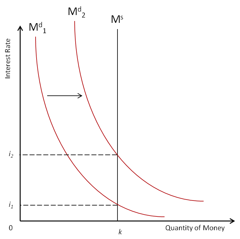
In the diagram above, Ms stands for money supplied and Md stands for money demanded. Ms is a straight line because the central bank can only produce a fixed amount of money at any point in time. Before the government borrowed money from the central bank, Md was at Md1, resulting in the interest rate being at i1. Once the government borrows more money from the central bank, Md increases to Md2, resulting in the interest rate shifting to i2.

Why doesn’t the central bank increase money supplied in order to decrease interest rates? A central bank can increase money supplied a limited number of times before inflation becomes uncontrollable.

b. When the government spends on roads and other such projects, it takes away the opportunity to build those projects from the private sector, thus crowding them out.

4. Consumer surplus

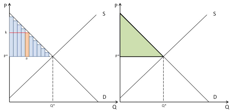
​Consumer surplus is the difference between the reservation price and the price paid for the good, i.e. the amount of benefit consumers get from buying the good. In the diagram below, consumer surplus for someone willing to spend $k is the difference between the reservation price, $k, and the market price, P*, illustrated by the red rectangle. Therefore, total consumer surplus is the area below the demand curve but above the market price, i.e. the green triangle.

Synopsis: Why productivity growth has slowed down and what to do about it

Click here to read the original article.

Discussion:

This article discusses the reason for a sluggish productivity growth. The OECD attributes this to a lack of “diffusion” – or spreading of innovation – to less innovative firms, thereby blocking productivity growth. Its suggested remedy is to intensify global competition in order to cut out the slow and old firms.

While some argue that the slow productivity may be attributed to the slowing pace of innovation in general, the OECD shows that top competitors of each sector are innovating now more than ever. Thus, the OECD research concludes that the petering of productivity could be a product of the distribution of innovation slowing down.

The reason why this distribution is not happening as quickly as before is due to the fact that “creative destruction” has lost its edge. This may be caused by increased government regulation, which traps workers in jobs for which they are overqualified. In turn, these unproductive firms tend to drag down aggregate productivity by absorbing valuable resources. This, in turn, reduces the growth of more innovative firms. Prime examples of this are Italy and Spain.

Key Terms:

1. Creative destruction is a famous concept by Austrian economist Joseph Schumpeter. The general idea is that creative destruction happens when something new destroys something old, like when the print media was destroyed by online news.

2. A zombie firm is a firm that needs constant support from the government (in the form of bailouts, etc.) to stay afloat. Without the help of the government, this firm would collapse. Japan had a number of zombie firms in its economy before its economic bubble burst and it slipped into depression. Although the number of zombie firms has drastically reduced since then, it still has an unusually high number of such firms.

Context:

1. This article states that one reason why slowing productivity growth is happening is because of “a slowing in the pace of productivity enhancing innovation”. Tyler Cowen, who is mentioned in an earlier blog post, discusses this idea in his book “The Great Stagnation”, saying that the ‘low hanging fruit’ of technological innovation (i.e. the obvious and easy to reach ones) have all been plucked, and innovating new technology will be much harder from now on.

2. The OECD research on the innovation of top firms in each sector begs the question: how do we measure productivity? My guess is that they measure the value of output divided by the number of workers.

3. The OECD claims that the “breakdown of the diffusion machine” has slowed productivity growth, but I would like to raise the question of whether or not there was a diffusion machine earlier that was working properly.

Synopsis: Paul Krugman provides a graphical representation of S.R.’s article, which discusses the flaws with the claim that China has wasted $6.8tn on investments.

Click here to read the original article.

Click here to read the blog post on S.R.'s article.

Discussion:
This article substantiates the article written by S.R. (found here), while pointing out the graphical representation of Mr. Xu and Mr. Wang’s paper and thus highlights the problem with their claims.

Krugman also adds that an increasing ICOR does not mean wasted investment; it just suggests diminishing marginal returns.

Context:
Looking at Figure 1, which describes diminishing returns as we move along the curve from A to B to C, we must notice that Krugman has used the axes titles “output per worker” and “capital per worker”. Why has he used per worker instead of “total output” and “total capital”? If the graph were to show “total output” and “total capital” with the same curve, the analysis would be as such: the reason why total output does not increase as total capital increases is because there aren’t enough workers to use the increasing amounts of capital. This does not show diminishing returns, it just shows inefficiency. If we measure both per worker, which standardises the unit between both axes, we can see diminishing returns.

Synopsis: Is China’s productivity slowing down?

Click here to read the original article

Discussion:
This article discusses the source and extent of China’s productivity slowdown. In other words, to a large extent, China’s slowing economy can be blamed on disappointing growths in productivity. For the past few decades, China’s boom was caused by an increase in labour and capital, as opposed to an increase in efficiency. The measure of where the source of GDP is from is TFP (total factor productivity), which is, according to the article, “subtracting the change in capital and labour deployed from the change in overall output.” I will discuss the problems with this statement later.

Between different people are differing opinions on China’s TFP. Mr. Harry Wu, an economist who has done a lot of research on the shortcomings of Chinese official data, has a pessimistic opinion (which, itself, faces a plethora of problems given the assumptions he made) and cites a negative TFP, while the World Bank’s more hopeful one shows a slowdown in TFP, even if it is positive for the time being.

Exacerbating China’s problem with a showdown of productivity is China’s bad lending and investment decisions. China’s best firms do not have the credit they deserve. With TFP and ICOR (explained later) increasing, China is likely to face large problems.

Key Words:
1.       ICOR: Incremental Capital-Output Ratio is the measure of how much investment is needed to increase growth by a percentage point.
2.       TFP: Total Factor Productivity, as I said earlier, is stated to be the difference between the change in capital and labour and the change in overall output. Math students will understand the problems with this statement. What does subtraction mean? (The figures in the following tables are not based on actual data).

Does this mean the TFP is 20%-10%=10%? Because this is what the article says. What I have calculated is the change in GDP and the change in input, and I have subtracted the two, as per the instructions of the article.

This is how TFP is actually calculated:

TFP Calculation 2:

So, the TFP is now 2.1818/2=9.09%

The difference between the two methods is that firstly, there is no subtraction in the second calculation, and secondly, it is not the change in GDP per year by the change in input per year as the first table would suggest, but rather, the change in ratio between GDP and input per year.

The difference between 9.09% and 10% from both tables might seem negligible, but on a large scale, this could make a large difference.

This is not to say that the writer did not understand how TFP was calculated; his or her phrasing was merely meant for readers to understand the general concept. I think it is important to notice these small differences, though.