Synopsis: The fourth in The Economist’s series on seminal economic ideas discusses the relevance and usefulness of the fiscal multiplier.
Click here to read the original article.
Click here to read the original article.
Discussion:
Introduction
The idea of the fiscal multiplier was first introduced after World War 1, and has since gained and lost popularity. Now, when economies around the world are debating the usefulness of fiscal stimulus in the face diminishing effectiveness in using monetary stimulus, economists have gone back to the age-old debate: are fiscal multipliers real?
The fiscal multiplier
The mathematics of the fiscal multiplier will be explained under ‘Context’.
The multiplier explains a scenario in which an initial increase (or decrease) in government spending will increase (or decrease) national income by a disproportionate amount.
For example, if the government spends money to build a new school, construction workers, architects, building planners, etc. will be involved in building it. Later, new teachers, janitors and other staff would get hired. The people involved in either building or running the school would then spend some (not all) of the money on other goods and services, such as restaurants. Now, people working at the restaurants have more income, and they can spend some of it on other goods and services, and so on. Thus, the initial action of increased government spending benefits the economy in many ways. The question is to what extent is the accumulated benefits of the successive waves of spending exceed the initial government expenditure.
History of the fiscal multiplier: the 1920s
Many times, the idea is credited to JM Keynes himself, but it was his student, Baron Kahn, who first mentioned it. In the late 1920s the U.K. had slipped into a recession, as World War 1 had caused a depreciation in the pound, while inflation was high. To counteract a low pound, the Bank of England maintained tight monetary control (explained under ‘Context’). This, in turn, created a period of persisting low growth and deflation – the Great Depression.
Many economists had suggested public investment to increase employment in the economy. This idea was unsurprisingly met with resistance from the government, which echoed the U.S. Treasury’s view: public spending would crowd out private spending (to read more about the crowding-out effect, click here), and thus would not help the economy. In fact, it might exacerbate the depression.
Baron Kahn argued vehemently against the “Treasury view”, stating that public investment would increase output not only from the primary spending, but also from “beneficial repercussions”.
The Keynesian multiplier and “General Theory”
Unsurprisingly, Kahn’s view was in line with that of his teacher. In his seminal work, “The General Theory of Employment, Interest and Money” (“GT”), Keynes described exactly how the multiplier would boost growth. Because of not only his thorough description of the concept, but also his influence globally, the fiscal multiplier is often referred to as the “Keynesian multiplier”.
GT was, and continues to be, one of the greatest pieces of economic writing. Keynes’ motivation to write the book stemmed from his frustration with the Treaty of Versailles: he lampooned key figures for not considering what he believed were large risks with the agreements set out in the treaty. Keynes, as well, was very unhappy with what was then considered common and accepted economic knowledge, i.e. classical economics (explained under context). Both these factors drove him to write what would be his magnum opus: GT.
It is in GT that Keynes describes the mechanism through which government spending would have secondary effects, which would lead to tertiary effects, and so on. He also states that during a recession, individuals would be more inclined to save than invest; thus, demand for investment would decrease. As a result, an increase in demand for investment from the government should not cause a crowding-out effect.
History of the fiscal multiplier: the 1920s to the 1960s
The success of the theory of fiscal multiplier seemed to be self-evident during the Second World War and for a long time after. The Great Depression prompted economies worldwide, especially the U.S. and the U.K., to adopt Keynesian economics, and the fiscal multiplier. As the governments eventually increased military spending in the course of World War II, their economies emerged from depression. Reverence of the multiplier increased multifold after, leading Milton Friedman to state, “We’re all Keynesians now”.
History of the fiscal multiplier: the 1970s
It was Friedman himself who began the long line of criticisms of the multiplier. He outlined the relationship between the business cycle and the money supply in an economy, and thus stated that controlling the money supply was all that was needed to control an economy; the multiplier was not necessary at all.
A more fierce line of criticism stemmed from economists belonging to the “rational expectations” school of thought, led by Robert Lucas. They claimed that the multiplier does not exist. Forward-looking individuals would realize that fiscal expansion today would have to be met with fiscal consolidation in the future to stabilize debt: thus, they would save the money they get from the government for when there is an increase in taxes in the future. Thus, there would be no multiplier effect. This idea is dubbed “Ricardian equivalence” (discussed under ‘Context’).
History of the fiscal multiplier: post-1970s
Governments tried fruitlessly to boost economic growth through government spending. Yet, they found that despite quiescent unemployment, inflation and interest rates rose unsustainably. The economic situation post-70s gave rise to a school of economic thought dubbed the “freshwater” school (these economists were named as such due to their proximity to the Great Lakes in the U.S.). They fought to recreate macroeconomics from individual consumers’ actions, a phenomenon named “microfoundations of macroeconomics”.
Robert Lucas’s and Tom Sargent’s work on the criticisms of Keynesian economics won them the Nobel Prize, and the fiscal multiplier quickly lost popularity and pertinence.
Then came the rise of “New Keynesian” economists, most of whom came from near America’s coasts; thus, they were dubbed “saltwater” economists. Notable saltwater economists include Larry Summers, Stanley Fischer and Greg Mankiw. New Keynesian economists believed that “recessions were market failures that could be fixed through government intervention”. However, they placed more importance on the central banks’ management of inflation, unemployment and interest rates than they did on fiscal policy. Thus, the fiscal multiplier once again faded into the background.
History of the fiscal multiplier: the 1990s to now
Developing countries around the world have been seeing little success in central bank policies, especially quantitative easing. Since the 1990s, inflation has remained close to being non-existent in Japan despite the Bank of Japan’s best efforts. Cutting interest rates to zero has not been as successful as any economy had hoped. This led to the resumption of the conversation about fiscal expansion. After the Global Financial Crisis (GFC), the U.S. had secured an $800bn stimulus package to revive its economy.
Freshwater economists argue that during times of panic, economists have resorted to the comforting idea of fiscal expansion, even when it doesn’t work. Other economists argue that the lack of fiscal stimulus after the GFC has damaged economies worldwide. Only time will tell which side of the argument is correct. The only thing that seems clear to economists now is that the argument about Keynes’ multiplier will never end.
Recent experiences or evidence
Fiscal multiplier has been calculated to be greater than one for many developed economies. This means that fiscal expansion will boost the economy past its primary effects, while austerity (fiscal consolidation) will harm the economy more than the initial amount of contraction.
In the EU: Austerity has been a centerpiece of government policy ever since the GFC. In the UK, former Prime Minister David Cameron mentioned the “age of austerity” in a 2009 speech to the Conservative Party. In March, the ex-Chancellor of the Exchequer George Osborne mentioned further government spending cuts of about £4bn. Austerity measures in the EU are well-summarized by this website. Some economists believe that it is excessive austerity measures across Europe that keep struggling economies from a full recession, and that the UK only escaped the recession after austerity measures were loosened.
In Japan: Prime Minister Shinzo Abe has been discussing his “three arrows” to economic recovery for a long time: monetary expansion, fiscal expansion and structural reforms (such as encouraging women to participate in the labor force). However, fiscal expansion has been constantly negated at least partially by increased taxation of sorts, including consumption tax and sales tax.
In the U.S.: The U.S. government, under President Barack Obama, had secured an $800bn fiscal expansion package after the GFC. This, along with QE, did well to aid the economic recovery from the recession. However, many economists such as Larry Summers argue that the fiscal expansion package was not large enough and a larger one would have pulled the U.S. out of recession much quicker.
Context
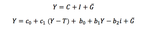
Assume a closed economy (i.e. one where there are no imports and exports). The output, denoted by Y, in the economy comes from three sections, each of which can be modeled as follows:
Together, then, total output (or GDP) in an economy is:
Introduction
The idea of the fiscal multiplier was first introduced after World War 1, and has since gained and lost popularity. Now, when economies around the world are debating the usefulness of fiscal stimulus in the face diminishing effectiveness in using monetary stimulus, economists have gone back to the age-old debate: are fiscal multipliers real?
The fiscal multiplier
The mathematics of the fiscal multiplier will be explained under ‘Context’.
The multiplier explains a scenario in which an initial increase (or decrease) in government spending will increase (or decrease) national income by a disproportionate amount.
For example, if the government spends money to build a new school, construction workers, architects, building planners, etc. will be involved in building it. Later, new teachers, janitors and other staff would get hired. The people involved in either building or running the school would then spend some (not all) of the money on other goods and services, such as restaurants. Now, people working at the restaurants have more income, and they can spend some of it on other goods and services, and so on. Thus, the initial action of increased government spending benefits the economy in many ways. The question is to what extent is the accumulated benefits of the successive waves of spending exceed the initial government expenditure.
History of the fiscal multiplier: the 1920s
Many times, the idea is credited to JM Keynes himself, but it was his student, Baron Kahn, who first mentioned it. In the late 1920s the U.K. had slipped into a recession, as World War 1 had caused a depreciation in the pound, while inflation was high. To counteract a low pound, the Bank of England maintained tight monetary control (explained under ‘Context’). This, in turn, created a period of persisting low growth and deflation – the Great Depression.
Many economists had suggested public investment to increase employment in the economy. This idea was unsurprisingly met with resistance from the government, which echoed the U.S. Treasury’s view: public spending would crowd out private spending (to read more about the crowding-out effect, click here), and thus would not help the economy. In fact, it might exacerbate the depression.
Baron Kahn argued vehemently against the “Treasury view”, stating that public investment would increase output not only from the primary spending, but also from “beneficial repercussions”.
The Keynesian multiplier and “General Theory”
Unsurprisingly, Kahn’s view was in line with that of his teacher. In his seminal work, “The General Theory of Employment, Interest and Money” (“GT”), Keynes described exactly how the multiplier would boost growth. Because of not only his thorough description of the concept, but also his influence globally, the fiscal multiplier is often referred to as the “Keynesian multiplier”.
GT was, and continues to be, one of the greatest pieces of economic writing. Keynes’ motivation to write the book stemmed from his frustration with the Treaty of Versailles: he lampooned key figures for not considering what he believed were large risks with the agreements set out in the treaty. Keynes, as well, was very unhappy with what was then considered common and accepted economic knowledge, i.e. classical economics (explained under context). Both these factors drove him to write what would be his magnum opus: GT.
It is in GT that Keynes describes the mechanism through which government spending would have secondary effects, which would lead to tertiary effects, and so on. He also states that during a recession, individuals would be more inclined to save than invest; thus, demand for investment would decrease. As a result, an increase in demand for investment from the government should not cause a crowding-out effect.
History of the fiscal multiplier: the 1920s to the 1960s
The success of the theory of fiscal multiplier seemed to be self-evident during the Second World War and for a long time after. The Great Depression prompted economies worldwide, especially the U.S. and the U.K., to adopt Keynesian economics, and the fiscal multiplier. As the governments eventually increased military spending in the course of World War II, their economies emerged from depression. Reverence of the multiplier increased multifold after, leading Milton Friedman to state, “We’re all Keynesians now”.
History of the fiscal multiplier: the 1970s
It was Friedman himself who began the long line of criticisms of the multiplier. He outlined the relationship between the business cycle and the money supply in an economy, and thus stated that controlling the money supply was all that was needed to control an economy; the multiplier was not necessary at all.
A more fierce line of criticism stemmed from economists belonging to the “rational expectations” school of thought, led by Robert Lucas. They claimed that the multiplier does not exist. Forward-looking individuals would realize that fiscal expansion today would have to be met with fiscal consolidation in the future to stabilize debt: thus, they would save the money they get from the government for when there is an increase in taxes in the future. Thus, there would be no multiplier effect. This idea is dubbed “Ricardian equivalence” (discussed under ‘Context’).
History of the fiscal multiplier: post-1970s
Governments tried fruitlessly to boost economic growth through government spending. Yet, they found that despite quiescent unemployment, inflation and interest rates rose unsustainably. The economic situation post-70s gave rise to a school of economic thought dubbed the “freshwater” school (these economists were named as such due to their proximity to the Great Lakes in the U.S.). They fought to recreate macroeconomics from individual consumers’ actions, a phenomenon named “microfoundations of macroeconomics”.
Robert Lucas’s and Tom Sargent’s work on the criticisms of Keynesian economics won them the Nobel Prize, and the fiscal multiplier quickly lost popularity and pertinence.
Then came the rise of “New Keynesian” economists, most of whom came from near America’s coasts; thus, they were dubbed “saltwater” economists. Notable saltwater economists include Larry Summers, Stanley Fischer and Greg Mankiw. New Keynesian economists believed that “recessions were market failures that could be fixed through government intervention”. However, they placed more importance on the central banks’ management of inflation, unemployment and interest rates than they did on fiscal policy. Thus, the fiscal multiplier once again faded into the background.
History of the fiscal multiplier: the 1990s to now
Developing countries around the world have been seeing little success in central bank policies, especially quantitative easing. Since the 1990s, inflation has remained close to being non-existent in Japan despite the Bank of Japan’s best efforts. Cutting interest rates to zero has not been as successful as any economy had hoped. This led to the resumption of the conversation about fiscal expansion. After the Global Financial Crisis (GFC), the U.S. had secured an $800bn stimulus package to revive its economy.
Freshwater economists argue that during times of panic, economists have resorted to the comforting idea of fiscal expansion, even when it doesn’t work. Other economists argue that the lack of fiscal stimulus after the GFC has damaged economies worldwide. Only time will tell which side of the argument is correct. The only thing that seems clear to economists now is that the argument about Keynes’ multiplier will never end.
Recent experiences or evidence
Fiscal multiplier has been calculated to be greater than one for many developed economies. This means that fiscal expansion will boost the economy past its primary effects, while austerity (fiscal consolidation) will harm the economy more than the initial amount of contraction.
In the EU: Austerity has been a centerpiece of government policy ever since the GFC. In the UK, former Prime Minister David Cameron mentioned the “age of austerity” in a 2009 speech to the Conservative Party. In March, the ex-Chancellor of the Exchequer George Osborne mentioned further government spending cuts of about £4bn. Austerity measures in the EU are well-summarized by this website. Some economists believe that it is excessive austerity measures across Europe that keep struggling economies from a full recession, and that the UK only escaped the recession after austerity measures were loosened.
In Japan: Prime Minister Shinzo Abe has been discussing his “three arrows” to economic recovery for a long time: monetary expansion, fiscal expansion and structural reforms (such as encouraging women to participate in the labor force). However, fiscal expansion has been constantly negated at least partially by increased taxation of sorts, including consumption tax and sales tax.
In the U.S.: The U.S. government, under President Barack Obama, had secured an $800bn fiscal expansion package after the GFC. This, along with QE, did well to aid the economic recovery from the recession. However, many economists such as Larry Summers argue that the fiscal expansion package was not large enough and a larger one would have pulled the U.S. out of recession much quicker.
Context
- What is the fiscal multiplier?
Assume a closed economy (i.e. one where there are no imports and exports). The output, denoted by Y, in the economy comes from three sections, each of which can be modeled as follows:
- Consumption, denoted by C. Consumption is written as , where:
- c0 is consumer confidence. The more confident a consumer is in the economy, the more the consumer will consume, i.e. the higher c0 is.
- (Y – T) is the disposable income. Y is the income a consumer earns, and T is the tax rate. Note that output is the same symbol as income. The intuition behind this is that all the income earned in an economy will finally be spent in the market, i.e. all the income will result in output. Thus, in this model, income = output. (Y – T) is then the disposable income for a consumer, i.e. the income a consumer can spend in the economy after taxes.
- c1 is the marginal propensity to consume (MPC). This is the share of disposable income that the consumer will actually spend in the economy. Whatever the consumer does not spend, he or she will save. For this reason, MPC is a figure between 0 and 1.
- Investment, denoted by I. Investment is written as , where:
- b0 is business confidence. The more confident a business is in the economy, the more the business will invest in the economy, i.e. the higher b0 is.
- b1Y is the proportion of output that leads to investment. In other words, a business that needs to make more and more output will invest more and more in machinery and other things. b1 denotes the proportion of increased output that results in increased investment. b1 always between 0 and 1.
- b2i is the amount by which an increase in interest rate results in a decrease in investment. If interest rates increase in an economy, it gets more expensive for a firm to borrow money to use in investments, such as machinery.
- Government spending, denoted by . The bar above the G denotes that government spending is exogenous, i.e. not determined by the market, but determined by the government itself.
Together, then, total output (or GDP) in an economy is:
Rearranging for Y on one side:
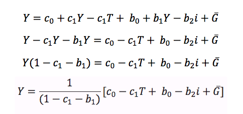
The fiscal multiplier is 1/(1-c1-b1). Thus, whatever happens to any term within the squared brackets, which we call autonomous spending, e.g. if government spending goes up or if taxes go down, Y will be affected through the fiscal multiplier, which would increase the effects of an increase in government spending or a decrease in taxes.
2. Why would the Bank of England’s maintaining tight monetary control counteract a low pound?
Tight monetary control means less money supply, which would keep both interest rates and currency value high.
Reducing the money supply in the domestic economy increases interest rates. This is demonstrated in the diagram below.
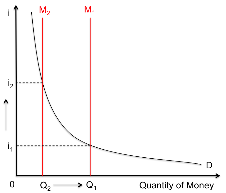
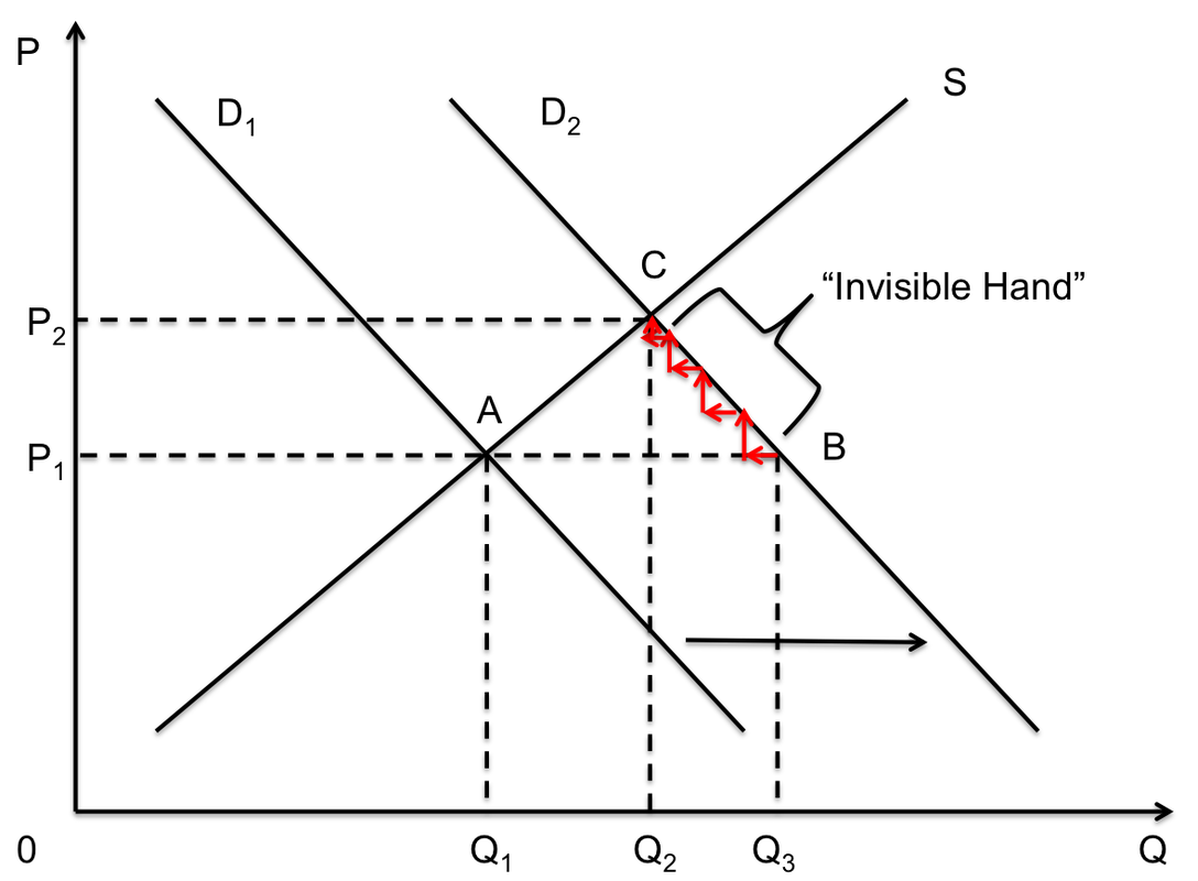
In this diagram, demand for money is denoted by D, and the original supply of money is M1. At the intersection of M1 and D, the quantity of money supplied is Q1, and the interest rate is i1. When the central bank reduces the stock of money, from M1 to M2, the quantity of money reduces to Q2, and the interest rate increases to i2, at the new equilibrium.
In the international market, reducing the stock of money increases the currency value. This is shown in the diagram below.
In the international market, reducing the stock of money increases the currency value. This is shown in the diagram below.

The demand for the British pound is denoted by D, and the original supply of the pound is S1. The equilibrium price and quantity of the pound at this equilibrium is P1 and P2 respectively. When the central bank reduces the amount of money supplied in the international markets, i.e. decreasing S1 to S2, at the new equilibrium, the quantity of pounds traded decreases to Q2 while the price increases to P2. Thus, the exchange rate increases.
3. Why was Keynes unhappy with classical economics?
Classical economists believed that the labor market is self-correcting, in that people who were not employed did not want to be employed. In other words, there is no such thing as involuntary unemployment.
3. Why was Keynes unhappy with classical economics?
Classical economists believed that the labor market is self-correcting, in that people who were not employed did not want to be employed. In other words, there is no such thing as involuntary unemployment.
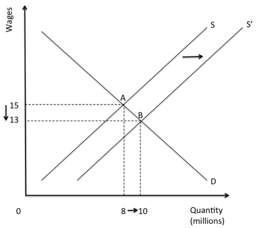
Consider a simple supply and demand diagram for the labor market, where S is the supply of labor and D is the demand for labor by employers. At the given market equilibrium, A, 8 million people are hired at a price of $15 an hour. Assume more people want to be hired, i.e. the supply of labor increased from S to S’. The new equilibrium is at point B, where 10 million people are hired. However, all laborers now get paid more, at $13 an hour.
This classical model of the labor market suggests that the economy can freely expand and contract to accommodate more or fewer workers, with no problem at all. This was the basic idea that Keynes disagreed with.
Keynes, instead, believed that individuals were more likely to accept more nominal wages rather than less nominal wages, even if their real wages did not change. In other words, prices of labor in the economy do not adjust as easily as classicists believed. He called this the “sticky wage” theorem.
Nominal wages is just the amount of money individuals earn. Real wages are adjusted to inflation. Now, suppose inflation in the economy increased by 2%, i.e. everything cost 2% more. Wages would increase by 2% as well. The individual who receives higher nominal wages is not richer by real terms, but is still happy. However, suppose there is 2% deflation in the economy, i.e. everything costs 2% less. An individual would be much less willing to receive a 2% pay cut, even if he or she remains equally as rich in real terms after the wage cut. Thus, wages are sticky downwards.
4. What are the problems with Richardian equivalence?
Ricardian equivalence requires that individuals are forward looking: they will save now for a future tax increase. However, few individuals are actually that forward looking, and those who are will not be able to accurately pinpoint when taxes will increase in the future. Thus, if individuals get a boost to their incomes due to higher government expenditure, they are more likely to spend at least a part of the increased income now and worry about tax increases later.
 RSS Feed
